Contributing

This example was automatically generated from a Jupyter notebook in the RxInferExamples.jl repository.

We welcome and encourage contributions! You can help by:

Improving this example
Creating new examples
Reporting issues or bugs
Suggesting enhancements

Visit our GitHub repository to get started. Together we can make RxInfer.jl even better! 💪

Autoregressive Active Inference

This example demonstrates an active inference agent that controls a thermal-coupled positioning stage while learning its physical parameters online. Both perception (Bayesian filtering) and action selection (expected free energy minimisation) are expressed as message passing on a shared factor graph — no separate controller is needed.

The agent design follows [1], which introduces message passing-based inference in an autoregressive active inference agent and evaluates it on robot navigation.

Navigation tip: node and rule definitions are in collapsible cells. To jump straight to the simulation, click here.

We begin by importing the required packages.

using RxInfer
using LinearAlgebra
using Distributions
using DomainSets
using Optim
using ForwardDiff
using SpecialFunctions
using StatsPlots
using Plots

import BayesBase
import FastCholesky: cholinv
import ExponentialFamily: MatrixNormalWishart
import StatsFuns: logmvgamma
import Random

default(label="", grid=false, markersize=3)
RxInfer.disable_inference_error_hint!()

1. Problem Statement

The thermal-coupled positioning stage is a force-driven 2D mechanical system with unknown mass $m$ and viscous damping $d$. A lumped thermal state $T$ heats up during operation (power input $P$) and cools toward ambient $T_\text{amb}$ at rate $\kappa$:

\[\dot{p} = v, \qquad m\dot{v} = u - d\,v, \qquad \dot{T} = -\kappa(T - T_\text{amb}) + \eta P.\]

What makes the task nontrivial is the observation model. The agent sees the end-effector in workpiece coordinates, which are thermally offset from the stage frame by an unknown thermal expansion coefficient $\alpha \in \mathbb{R}^2$:

\[y_k = p_k + \alpha\,(T_k - T_\text{amb}) + \varepsilon_k.\]

As the stage heats up, workpiece observations drift even without any applied force. The agent must navigate the end-effector through a sequence of workpiece-frame waypoints while compensating for this drift — without ever observing $T$ or knowing $\alpha$.

mutable struct ThermalStage
    mass    :: Float64
    damping :: Float64
    alpha   :: Vector{Float64}   # thermal expansion coefficient (unknown to agent)
    kappa   :: Float64            # cooling rate
    eta     :: Float64            # heat-input efficiency
    T_amb   :: Float64
    P_proc  :: Float64            # operating power
    sigma_obs :: Float64          # observation noise std (workpiece frame)
    sigma_v   :: Float64          # process noise on velocity
    sigma_T   :: Float64          # thermal process noise
    dt      :: Float64
    p :: Vector{Float64}          # stage position (true, unobserved)
    v :: Vector{Float64}          # stage velocity (true, unobserved)
    T :: Float64                  # thermal state  (true, unobserved)
    function ThermalStage(; mass=1.0, damping=0.5, alpha=[0.1, 0.05],
                            kappa=0.1, eta=1.0, T_amb=0.0, P_proc=1.0,
                            sigma_obs=1e-3, sigma_v=1e-3, sigma_T=1e-3, dt=0.1)
        new(mass, damping, alpha, kappa, eta, T_amb, P_proc,
            sigma_obs, sigma_v, sigma_T, dt, zeros(2), zeros(2), T_amb)
    end
end

function stage_step!(env::ThermalStage, u::Vector, process::Bool=false)
    dt  = env.dt
    a   = (u .- env.damping .* env.v) ./ env.mass
    env.v = env.v + dt .* a   + env.sigma_v .* randn(2)
    env.p = env.p + dt .* env.v
    P     = process ? env.P_proc : 0.0
    env.T = env.T + dt * (-env.kappa * (env.T - env.T_amb) + env.eta * P) + env.sigma_T * randn()
    return env.p + env.alpha .* (env.T - env.T_amb) + env.sigma_obs .* randn(2)
end

stage_step! (generic function with 2 methods)

2. Agent Specification

The agent maintains a probabilistic model of its own dynamics and selects actions by minimising expected free energy (EFE). Both the model update (filtering) and action selection (planning) reduce to message passing on the same factor graph structure.

2.1 Generative Model

The stage dynamics are approximated by a Multivariate AutoRegressive model with eXogenous inputs (MARX) [1]. Writing the regressor as

\[x_k = \begin{bmatrix} y_{k-1} \\ y_{k-2} \\ u_k \\ u_{k-1} \\ u_{k-2} \end{bmatrix},\]

the next workpiece-frame observation follows $y_k = M^\top x_k + \text{noise}$, where the parameter matrix $M$ and the noise precision jointly have a Matrix-Normal-Wishart prior $\Phi \sim \mathrm{MNW}(M_0, U_0, V_0, \nu_0)$. Updating $\Phi$ from data gives online estimates of mass, damping, and thermal expansion — all absorbed into $M$.

The regressor buffers (backshift) and numerical stabilisation (proj2psd) are collected in the hidden cell below.

Hidden block of utility functions: backshift, proj2psd, and MatrixNormalWishart product override - click to expand


function backshift(x::AbstractVector, a::Number)
    N = size(x, 1)
    S = Tridiagonal(ones(N - 1), zeros(N), zeros(N - 1))
    e = [1.0; zeros(N - 1)]
    return S * x + e * a
end
backshift(M::AbstractMatrix, a::Number) = diagm(backshift(diag(M), a))
backshift(x::AbstractMatrix, a::Vector) = [a x[:, 1:end-1]]

function proj2psd(S::AbstractMatrix)
    L, V = eigen(S)
    S = V * diagm(max.(1e-8, L)) * V'
    return (S + S') / 2
end

# After many MARX learning steps the Ml'*ΛlMl + Mr'*ΛrMr - rhs'*M terms grow large
# (~1e4), and floating-point cancellation yields |Ω[i,j] - Ω[j,i]| > 1e-8 absolute,
# which triggers FastCholesky's CI check. Wrapping matrices with Symmetric() before
# each Cholesky ensures the check passes and future cholinv calls on stored U/V do too.
function BayesBase.prod(::BayesBase.PreserveTypeProd{Distribution}, left::MatrixNormalWishart, right::MatrixNormalWishart)
    Ml, Ul, Vl, νl = BayesBase.params(left)
    Mr, Ur, Vr, νr = BayesBase.params(right)
    Λl = cholinv(Symmetric(Ul)); Λr = cholinv(Symmetric(Ur)); Λ = Λl + Λr
    U  = cholinv(Symmetric(Λ))
    ΛlMl = Λl*Ml; ΛrMr = Λr*Mr; rhs = ΛlMl + ΛrMr; M = U*rhs
    Ωl = cholinv(Symmetric(Vl)); Ωr = cholinv(Symmetric(Vr))
    Ω  = Ωl + Ωr + Ml'*ΛlMl + Mr'*ΛrMr - rhs'*M
    V  = cholinv(Symmetric(Ω))
    n, p = size(Ml); ν = νl + νr + n - p - 1
    return MatrixNormalWishart(M, Symmetric(U), Symmetric(V), ν)
end

During planning, the message arriving at an action variable from the future is proportional to $\exp(-G(u))$, where $G(u)$ is the EFE of taking action $u$. We represent it with a custom unBoltzmann distribution whose mode (the EFE-minimising action) is found by bounded L-BFGS optimisation seeded from the best box corner.

Hidden block of unBoltzmann distribution, its mode, and product rules - click to expand


struct unBoltzmann <: ContinuousMultivariateDistribution
    G::Function     # energy function (expected free energy over actions)
    N::Integer      # number of inputs
    D::Rectangle    # box support
    unBoltzmann(G::Function, N::Integer, D::Rectangle) = new(G, N, D)
end

BayesBase.ndims(d::unBoltzmann)   = d.N
BayesBase.support(d::unBoltzmann) = d.D

function BayesBase.mode(dist::unBoltzmann; time_limit=0.2, iterations=100)
    lo = support(dist).a; hi = support(dist).b; N = dist.N
    eps = 1e-6
    best_u = lo .+ eps; best_G = Inf
    for bits in Iterators.product(fill((0, 1), N)...)
        c = [bits[i] == 0 ? lo[i] + eps : hi[i] - eps for i in 1:N]
        g = dist.G(c)
        if isfinite(g) && g < best_G; best_G = g; best_u = c; end
    end
    opts = Optim.Options(time_limit=time_limit, allow_f_increases=true,
                         outer_iterations=iterations, iterations=1)
    gradG(J, u) = ForwardDiff.gradient!(J, dist.G, u)
    results = optimize(dist.G, gradG, lo, hi, best_u, Fminbox(LBFGS()), opts)
    return Optim.minimizer(results)
end

BayesBase.cov(dist::unBoltzmann)       = inv(precision(dist))
BayesBase.precision(dist::unBoltzmann) = proj2psd(ForwardDiff.hessian(dist.G, mode(dist)))
pdf(dist::unBoltzmann, u::Vector)      = exp(-dist.G(u))
Distributions.logpdf(dist::unBoltzmann, u::Vector) = -dist.G(u)

BayesBase.default_prod_rule(::Type{<:unBoltzmann}, ::Type{<:unBoltzmann})      = BayesBase.ClosedProd()
BayesBase.default_prod_rule(::Type{<:AbstractMvNormal}, ::Type{<:unBoltzmann}) = BayesBase.ClosedProd()
BayesBase.default_prod_rule(::Type{<:unBoltzmann}, ::Type{<:AbstractMvNormal}) = BayesBase.ClosedProd()

function BayesBase.prod(::BayesBase.ClosedProd, left::unBoltzmann, right::unBoltzmann)
    left.N != right.N && error("Dimensionalities of energy functions do not match.")
    G(u) = left.G(u) + right.G(u)
    return unBoltzmann(G, right.N, intersectdomain(left.D, right.D))
end
function BayesBase.prod(::BayesBase.ClosedProd, left::AbstractMvNormal, right::unBoltzmann)
    ndims(left) != right.N && error("Dimensionality mismatch.")
    G(u) = -BayesBase.logpdf(left, u) + right.G(u)
    return unBoltzmann(G, right.N, right.D)
end
BayesBase.prod(::BayesBase.ClosedProd, left::unBoltzmann, right::AbstractMvNormal) = BayesBase.prod(BayesBase.ClosedProd(), right, left)

With a Matrix-Normal-Wishart prior over $\Phi$, the posterior predictive of the next observation is a multivariate Student's-t. We implement it as MvLocationScaleT(η, μ, Σ) with degrees of freedom $\eta$, location $\mu$, and scale $\Sigma$.

Hidden block of MvLocationScaleT distribution and product rules - click to expand


struct MvLocationScaleT{T,N<:Real,M<:AbstractVector{T},S<:AbstractMatrix{T}} <: ContinuousMultivariateDistribution
    η::N; μ::M; Σ::S
    function MvLocationScaleT(η::N, μ::M, Σ::S) where {T,N<:Real,M<:AbstractVector{T},S<:AbstractMatrix{T}}
        dims = length(μ)
        η <= dims && error("Degrees of freedom must exceed the dimensionality.")
        dims !== size(Σ, 1) && error("Dimensionalities of mean and covariance do not match.")
        return new{T,N,M,S}(η, μ, Σ)
    end
end

BayesBase.params(p::MvLocationScaleT)    = (p.η, p.μ, p.Σ)
BayesBase.ndims(p::MvLocationScaleT)     = length(p.μ)
BayesBase.mean(p::MvLocationScaleT)      = p.μ
BayesBase.mode(p::MvLocationScaleT)      = p.μ
BayesBase.cov(p::MvLocationScaleT)       = p.η > 2 ? p.η / (p.η - 2) * p.Σ : error("Degrees of freedom must exceed 2.")
BayesBase.precision(p::MvLocationScaleT) = inv(cov(p))

function pdf(p::MvLocationScaleT, x::Vector)
    d = ndims(p); η, μ, Σ = params(p)
    return sqrt(1 / ((η * π)^d * det(Σ))) * gamma((η + d) / 2) / gamma(η / 2) * (1 + 1 / η * (x - μ)' * inv(Σ) * (x - μ))^(-(η + d) / 2)
end
function Distributions.logpdf(p::MvLocationScaleT, x::Vector)
    d = ndims(p); η, μ, Σ = params(p)
    return -d / 2 * log(η * π) - 1 / 2 * logdet(Σ) + loggamma((η + d) / 2) - loggamma(η / 2) - (η + d) / 2 * log(1 + 1 / η * (x - μ)' * inv(Σ) * (x - μ))
end

BayesBase.default_prod_rule(::Type{<:MvLocationScaleT}, ::Type{<:MvLocationScaleT}) = BayesBase.ClosedProd()
BayesBase.default_prod_rule(::Type{<:AbstractMvNormal}, ::Type{<:MvLocationScaleT}) = BayesBase.ClosedProd()
BayesBase.default_prod_rule(::Type{<:MvLocationScaleT}, ::Type{<:AbstractMvNormal}) = BayesBase.ClosedProd()
BayesBase.default_prod_rule(::Type{<:MvLocationScaleT}, ::Type{<:unBoltzmann})      = BayesBase.ClosedProd()
BayesBase.default_prod_rule(::Type{<:unBoltzmann}, ::Type{<:MvLocationScaleT})      = BayesBase.ClosedProd()

function BayesBase.prod(::BayesBase.ClosedProd, left::MvLocationScaleT, right::MvLocationScaleT)
    ndims(left) != ndims(right) && error("Dimensionality mismatch.")
    ηl, μl, Σl = params(left); ηr, μr, Σr = params(right)
    Λl = inv(ηl / (ηl - 2) * Σl); Λr = inv(ηr / (ηr - 2) * Σr)
    Σ = inv(Λl + Λr); μ = Σ * (Λl * μl + Λr * μr)
    return MvNormalMeanCovariance(μ, Σ)
end
function BayesBase.prod(::BayesBase.ClosedProd, left::AbstractMvNormal, right::MvLocationScaleT)
    ndims(left) != ndims(right) && error("Dimensionality mismatch.")
    μl, Σl = mean_cov(left); ηr, μr, Σr = params(right)
    Λl = inv(Σl); Λr = inv(ηr / (ηr - 2) * Σr)
    Σ = inv(Λl + Λr); μ = Σ * (Λl * μl + Λr * μr)
    return MvNormalMeanCovariance(μ, Σ)
end
BayesBase.prod(::BayesBase.ClosedProd, left::MvLocationScaleT, right::AbstractMvNormal) = BayesBase.prod(BayesBase.ClosedProd(), right, left)
function BayesBase.prod(::BayesBase.ClosedProd, left::MvLocationScaleT, right::unBoltzmann)
    ndims(left) != ndims(right) && error("Dimensionality mismatch.")
    opts = Optim.Options(time_limit=1.0, allow_f_increases=true, iterations=10)
    Q(y) = -logpdf(left, y) - right.G(y)
    gradQ(J, y) = ForwardDiff.gradient!(J, Q, y)
    results = optimize(Q, gradQ, mean(left), LBFGS(), opts)
    y_map = Optim.minimizer(results)
    P_lap = proj2psd(ForwardDiff.hessian(Q, y_map))
    return MvNormalMeanPrecision(y_map, P_lap)
end
BayesBase.prod(::BayesBase.ClosedProd, left::unBoltzmann, right::MvLocationScaleT) = BayesBase.prod(BayesBase.ClosedProd(), right, left)

The MARX node is declared as a stochastic node with seven edges. The message passing rules are split by direction: the :Φ rule updates the parameter belief from a completed transition, the :out/:outprev rules compute the posterior-predictive Student's-t, and the :in/:inprev rules compute the EFE message towards actions.

Hidden block of MARX node declaration and MvLocationScaleT output rule - click to expand


struct MARX end
@node MARX Stochastic [out, outprev1, outprev2, in, inprev1, inprev2, Φ]

@rule MvLocationScaleT(:out, Marginalisation) (q_ν::PointMass, q_μ::PointMass, q_σ::PointMass) = begin
    return MvLocationScaleT(q_ν, q_μ, q_σ)
end

Parameter-learning rule (`:Φ`)

Given a fully observed transition, the message towards $\Phi$ is the Matrix-Normal-Wishart sufficient-statistic update of one regression datapoint.

Hidden block of MARX :Φ parameter-learning rules - click to expand



@rule MARX(:Φ, Marginalisation) (q_out::PointMass,
                                 q_outprev1::PointMass, 
                                 q_outprev2::PointMass, 
                                 q_in::PointMass, 
                                 q_inprev1::PointMass, 
                                 q_inprev2::PointMass) = begin

    y_k = mean(q_out)                                
    x_k = [mean(q_outprev1); mean(q_outprev2); mean(q_in); mean(q_inprev1); mean(q_inprev2)]

    Dy = length(y_k)
    Dx = length(x_k)

    Λ_ = x_k*x_k' + diagm(1e-8*ones(Dx))
    U_ = inv(Λ_)
    M_ = U_*(x_k*y_k')
    V_ = inv(diagm(1e-8*ones(Dy)))
    ν_ = 2 - Dx + Dy

    return MatrixNormalWishart(M_, U_, V_, ν_)
end

@rule MARX(:Φ, Marginalisation) (m_out::AbstractMvNormal,
                                 m_outprev1::Union{PointMass,AbstractMvNormal,MvLocationScaleT},
                                 q_outprev2::PointMass,
                                 m_in::Union{PointMass,AbstractMvNormal,unBoltzmann},
                                 m_inprev1::Union{PointMass,AbstractMvNormal,unBoltzmann}, 
                                 q_inprev2::PointMass) = begin

    return Uninformative()
end

@rule MARX(:Φ, Marginalisation) (m_out::AbstractMvNormal,
                                 m_outprev1::Union{PointMass,AbstractMvNormal,MvLocationScaleT},
                                 m_outprev2::Union{PointMass,AbstractMvNormal},
                                 m_in::AbstractMvNormal, 
                                 m_inprev1::Union{PointMass,AbstractMvNormal,unBoltzmann}, 
                                 m_inprev2::Union{PointMass,AbstractMvNormal,unBoltzmann}) = begin

    return Uninformative()
end

@rule MARX(:Φ, Marginalisation) (m_out::AbstractMvNormal, 
                                 q_outprev1::PointMass, 
                                 q_outprev2::PointMass, 
                                 m_in::Union{PointMass,AbstractMvNormal,unBoltzmann}, 
                                 q_inprev1::PointMass, 
                                 q_inprev2::PointMass, ) = begin 
    return Uninformative()
end

@rule MARX(:Φ, Marginalisation) (q_out::Union{AbstractMvNormal,unBoltzmann}, 
                                 q_outprev1::Union{PointMass,AbstractMvNormal,unBoltzmann},
                                 q_outprev2::Union{PointMass,AbstractMvNormal,unBoltzmann}, 
                                 q_in::Union{PointMass,AbstractMvNormal,unBoltzmann}, 
                                 q_inprev1::Union{PointMass,AbstractMvNormal,unBoltzmann}, 
                                 q_inprev2::Union{PointMass,AbstractMvNormal,unBoltzmann}, ) = begin 
    return Uninformative()
end

Prediction rules (`:out`, `:outprev`)

These rules return the posterior-predictive multivariate Student's-t of an output given the parameter belief and the rest of the regressor. With posterior $\Phi=(M,U,V,\nu)$ and regressor $x$, the predictive is $\mathrm{T}_{\nu-D_y+1}\!\big(M^\top x,\ \tfrac{1+x^\top U x}{\nu-D_y+1}V^{-1}\big)$.

Hidden block of MARX :out / :outprev message rules - click to expand


@rule MARX(:out, Marginalisation) (q_outprev1::Union{PointMass,AbstractMvNormal},
                                   q_outprev2::Union{PointMass,AbstractMvNormal}, 
                                   q_in::PointMass,
                                   q_inprev1::PointMass, 
                                   q_inprev2::PointMass,
                                   m_Φ::MatrixNormalWishart) = begin

    M,Λ,Ω,ν = params(m_Φ); Λ = inv(Λ); Ω = inv(Ω)

    x = [mode(q_outprev1); mode(q_outprev2); mode(q_in); mode(q_inprev1); mode(q_inprev2)]

    η = ν - Dy + 1
    μ = M'*x
    Σ = 1/(ν-Dy+1)*Ω*(1 + x'*inv(Λ)*x)
      
    return MvLocationScaleT(η,μ,Σ)
end

@rule MARX(:out, Marginalisation) (q_outprev1::PointMass, 
                                   q_outprev2::PointMass, 
                                   m_in::unBoltzmann,
                                   q_inprev1::PointMass, 
                                   q_inprev2::PointMass,
                                   m_Φ::MatrixNormalWishart,) = begin 

    M,Λ,Ω,ν = params(m_Φ); Λ = inv(Λ); Ω = inv(Ω)

    x = [mode(q_outprev1); mode(q_outprev2); mode(m_in); mode(q_inprev1); mode(q_inprev2)]

    η = ν - Dy + 1
    μ = M'*x
    Σ = 1/(ν-Dy+1)*Ω*(1 + x'*inv(Λ)*x)
    
    return MvLocationScaleT(η,μ,Σ)
end

@rule MARX(:out, Marginalisation) (m_outprev1::Union{AbstractMvNormal,MvLocationScaleT}, 
                                   q_outprev2::PointMass,
                                   m_in::Union{AbstractMvNormal,unBoltzmann},
                                   m_inprev1::Union{PointMass,unBoltzmann}, 
                                   q_inprev2::Union{PointMass,unBoltzmann},
                                   m_Φ::MatrixNormalWishart,) = begin 

    M,Λ,Ω,ν = params(m_Φ); Λ = inv(Λ); Ω = inv(Ω)

    x = [mode(m_outprev1); mode(q_outprev2); mode(m_in); mode(m_inprev1); mode(q_inprev2)]

    η = ν - Dy + 1
    μ = M'*x
    Σ = 1/(ν-Dy+1)*Ω*(1 + x'*inv(Λ)*x)
    
    return MvLocationScaleT(η,μ,Σ)
end

@rule MARX(:out, Marginalisation) (m_outprev1::Union{AbstractMvNormal,MvLocationScaleT}, 
                                   m_outprev2::Union{AbstractMvNormal,MvLocationScaleT},
                                   m_in::Union{AbstractMvNormal,MvLocationScaleT,unBoltzmann}, 
                                   m_inprev1::Union{AbstractMvNormal,MvLocationScaleT,unBoltzmann}, 
                                   m_inprev2::Union{AbstractMvNormal,MvLocationScaleT,unBoltzmann},
                                   m_Φ::MatrixNormalWishart,) = begin 

    M,Λ,Ω,ν = params(m_Φ); Λ = inv(Λ); Ω = inv(Ω)

    x = [mode(m_outprev1); mode(m_outprev2); mode(m_in); mode(m_inprev1); mode(m_inprev2)]

    η = ν - Dy + 1
    μ = M'*x
    Σ = 1/(ν-Dy+1)*Ω*(1 + x'*inv(Λ)*x)
    
    return MvLocationScaleT(η,μ,Σ)
end

@rule MARX(:out, Marginalisation) (q_outprev1::Union{PointMass,AbstractMvNormal,unBoltzmann}, 
                                   q_outprev2::Union{PointMass,AbstractMvNormal,unBoltzmann}, 
                                   q_in::Union{PointMass,AbstractMvNormal,unBoltzmann}, 
                                   q_inprev1::Union{PointMass,AbstractMvNormal,unBoltzmann}, 
                                   q_inprev2::Union{PointMass,AbstractMvNormal,unBoltzmann}, 
                                   q_Φ::MatrixNormalWishart, ) = begin
    M,Λ,Ω,ν = params(q_Φ); Λ = inv(Λ); Ω = inv(Ω)

    x = [mode(q_outprev1); mode(q_outprev2); mode(q_in); mode(q_inprev1); mode(q_inprev2)]

    η = ν - Dy + 1
    μ = M'*x
    Σ = 1/(ν-Dy+1)*Ω*(1 + x'*inv(Λ)*x)

    return MvLocationScaleT(η,μ,Σ)
end                                   

@rule MARX(:outprev1, Marginalisation) (q_out::unBoltzmann, 
                                        q_outprev2::PointMass, 
                                        q_in::unBoltzmann, 
                                        q_inprev1::AbstractMvNormal, 
                                        q_inprev2::PointMass, 
                                        q_Φ::MatrixNormalWishart, ) = begin

    M,Λ,Ω,ν = params(q_Φ); Λ = inv(Λ); Ω = inv(Ω)
    m_star  = mode(q_out)
    Du = length(mode(q_in))
    
    function G(outprev1)

        x = [outprev1; mode(q_outprev2); mode(q_in); mode(q_inprev1); mode(q_inprev2)]

        η = ν - Dy + 1
        μ = M'*x
        Σ = 1/(ν-Dy+1)*Ω*(1 + x'*inv(Λ)*x)
        return logpdf(MvLocationScaleT(η,μ,Σ), m_star)
    end
    return unBoltzmann(G,Dy,ProductDomain([(-Inf..Inf) for i in 1:Du]))                                
end

@rule MARX(:outprev1, Marginalisation) (q_out::unBoltzmann, 
                                        q_outprev2::PointMass, 
                                        q_in::unBoltzmann, 
                                        q_inprev1::unBoltzmann, 
                                        q_inprev2::PointMass, 
                                        q_Φ::MatrixNormalWishart, ) = begin        
    
    M,Λ,Ω,ν = params(q_Φ); Λ = inv(Λ); Ω = inv(Ω)
    m_star  = mode(q_out)
    Du = length(mode(q_in))
    
    function G(outprev1)

        x = [outprev1; mode(q_outprev2); mode(q_in); mode(q_inprev1); mode(q_inprev2)]

        η = ν - Dy + 1
        μ = M'*x
        Σ = 1/(ν-Dy+1)*Ω*(1 + x'*inv(Λ)*x)
        return logpdf(MvLocationScaleT(η,μ,Σ), m_star)
    end
    return unBoltzmann(G,Dy,ProductDomain([(-Inf..Inf) for i in 1:Du]))
end                                           

@rule MARX(:outprev1, Marginalisation) (q_out::Union{AbstractMvNormal,MvLocationScaleT}, 
                                        q_outprev2::Union{PointMass,AbstractMvNormal}, 
                                        q_in::Union{PointMass,AbstractMvNormal},
                                        q_inprev1::Union{PointMass,AbstractMvNormal}, 
                                        q_inprev2::Union{PointMass,AbstractMvNormal},
                                        m_Φ::MatrixNormalWishart) = begin
 
    M,Λ,Ω,ν = params(m_Φ); Λ = inv(Λ); Ω = inv(Ω)
    m_star  = mean(q_out)
    Du = length(mode(q_in))
    
    function G(outprev1)

        x = [outprev1; mode(q_outprev2); mode(q_in); mode(q_inprev1); mode(q_inprev2)]

        η = ν - Dy + 1
        μ = M'*x
        Σ = 1/(ν-Dy+1)*Ω*(1 + x'*inv(Λ)*x)
        return logpdf(MvLocationScaleT(η,μ,Σ), m_star)
    end
    return unBoltzmann(G,Dy,ProductDomain([(-Inf..Inf) for i in 1:Du]))
end

@rule MARX(:outprev1, Marginalisation) (q_out::Union{PointMass,AbstractMvNormal,unBoltzmann}, 
                                        q_outprev2::Union{PointMass,AbstractMvNormal}, 
                                        q_in::Union{PointMass,unBoltzmann,AbstractMvNormal}, 
                                        q_inprev1::Union{PointMass,unBoltzmann,AbstractMvNormal}, 
                                        q_inprev2::Union{PointMass,unBoltzmann,AbstractMvNormal}, 
                                        q_Φ::MatrixNormalWishart, ) = begin 

    M,Λ,Ω,ν = params(q_Φ); Λ = inv(Λ); Ω = inv(Ω)
    m_star  = mode(q_out)
    Du = length(mode(q_in))
    
    function G(outprev1)

        x = [outprev1; mode(q_outprev2); mode(q_in); mode(q_inprev1); mode(q_inprev2)]

        η = ν - Dy + 1
        μ = M'*x
        Σ = 1/(ν-Dy+1)*Ω*(1 + x'*inv(Λ)*x)
        return logpdf(MvLocationScaleT(η,μ,Σ), m_star)
    end
    return unBoltzmann(G,Dy,ProductDomain([(-Inf..Inf) for i in 1:Du]))
end

@rule MARX(:outprev1, Marginalisation) (m_out::Union{AbstractMvNormal,MvLocationScaleT}, 
                                        q_outprev2::Union{PointMass,AbstractMvNormal}, 
                                        m_in::Union{PointMass,AbstractMvNormal},
                                        m_inprev1::Union{PointMass,unBoltzmann}, 
                                        q_inprev2::Union{PointMass,unBoltzmann},
                                        m_Φ::MatrixNormalWishart) = begin

    M,Λ,Ω,ν = params(m_Φ); Λ = inv(Λ); Ω = inv(Ω)
    m_star  = mean(m_out)
    Du = length(mode(m_in))
    
    function G(outprev1)

        x = [outprev1; mode(q_outprev2); mode(m_in); mode(m_inprev1); mode(q_inprev2)]

        η = ν - Dy + 1
        μ = M'*x
        Σ = 1/(ν-Dy+1)*Ω*(1 + x'*inv(Λ)*x)
        return logpdf(MvLocationScaleT(η,μ,Σ), m_star)
    end
    return unBoltzmann(G,Dy,ProductDomain([(-Inf..Inf) for i in 1:Du]))
end

@rule MARX(:outprev1, Marginalisation) (m_out::AbstractMvNormal, 
                                        m_outprev2::AbstractMvNormal, 
                                        m_in::AbstractMvNormal, 
                                        m_inprev1::AbstractMvNormal, 
                                        m_inprev2::AbstractMvNormal, 
                                        m_Φ::MatrixNormalWishart, ) = begin 
    
    M,Λ,Ω,ν = params(m_Φ); Λ = inv(Λ); Ω = inv(Ω)
    m_star  = mean(m_out)
    Du = length(mode(m_in))
    
    function G(outprev1)

        x = [outprev1; mode(m_outprev2); mode(m_in); mode(q_inprev1); mode(q_inprev2)]

        η = ν - Dy + 1
        μ = M'*x
        Σ = 1/(ν-Dy+1)*Ω*(1 + x'*inv(Λ)*x)
        return logpdf(MvLocationScaleT(η,μ,Σ), m_star)
    end
    return unBoltzmann(G,Dy,ProductDomain([(-Inf..Inf) for i in 1:Du]))
end

@rule MARX(:outprev1, Marginalisation) (m_out::MvNormalMeanCovariance, 
                                        q_outprev2::PointMass, 
                                        m_in::Union{PointMass,unBoltzmann}, 
                                        m_inprev1::Union{PointMass,unBoltzmann}, 
                                        q_inprev2::Union{PointMass,unBoltzmann},
                                        m_Φ::MatrixNormalWishart,) = begin 
    
    M,Λ,Ω,ν = params(m_Φ); Λ = inv(Λ); Ω = inv(Ω)
    m_star  = mean(m_out)
    Du = length(mode(m_in))
    
    function G(outprev1)

        x = [outprev1; mode(q_outprev2); mode(m_in); mode(m_inprev1); mode(q_inprev2)]

        η = ν - Dy + 1
        μ = M'*x
        Σ = 1/(ν-Dy+1)*Ω*(1 + x'*inv(Λ)*x)
        return logpdf(MvLocationScaleT(η,μ,Σ), m_star)
    end
    return unBoltzmann(G,Dy,ProductDomain([(-Inf..Inf) for i in 1:Du]))
end

@rule MARX(:outprev1, Marginalisation) (m_out::AbstractMvNormal, 
                                        m_outprev2::AbstractMvNormal, 
                                        m_in::AbstractMvNormal, 
                                        m_inprev1::Union{PointMass,unBoltzmann}, 
                                        m_inprev2::Union{PointMass,unBoltzmann}, 
                                        m_Φ::MatrixNormalWishart, ) = begin 

    M,Λ,Ω,ν = params(m_Φ); Λ = inv(Λ); Ω = inv(Ω)
    m_star  = mean(m_out)
    Du = length(mode(m_in))
    
    function G(outprev1)

        x = [outprev1; mode(m_outprev2); mode(m_in); mode(m_inprev1); mode(m_inprev2)]

        η = ν - Dy + 1
        μ = M'*x
        Σ = 1/(ν-Dy+1)*Ω*(1 + x'*inv(Λ)*x)
        return logpdf(MvLocationScaleT(η,μ,Σ), m_star)
    end
    return unBoltzmann(G,Dy,ProductDomain([(-Inf..Inf) for i in 1:Du]))
end

@rule MARX(:outprev2, Marginalisation) (q_out::AbstractMvNormal, 
                                        q_outprev1::unBoltzmann, 
                                        q_in::Union{PointMass,unBoltzmann}, 
                                        q_inprev1::Union{PointMass,unBoltzmann}, 
                                        q_inprev2::Union{PointMass,AbstractMvNormal}, 
                                        q_Φ::MatrixNormalWishart, ) = begin
    return Uninformative()
end

@rule MARX(:outprev2, Marginalisation) (m_out::AbstractMvNormal, 
                                        m_outprev1::AbstractMvNormal, 
                                        m_in::AbstractMvNormal, 
                                        m_inprev1::AbstractMvNormal, 
                                        m_inprev2::AbstractMvNormal, 
                                        m_Φ::MatrixNormalWishart, ) = begin 
    

    

      
    return Uninformative()
end

@rule MARX(:outprev2, Marginalisation) (m_out::AbstractMvNormal, 
                                        m_outprev1::AbstractMvNormal, 
                                        m_in::AbstractMvNormal, 
                                        m_inprev1::unBoltzmann, 
                                        m_inprev2::unBoltzmann, 
                                        m_Φ::MatrixNormalWishart, ) = begin 
    

    

      
    return Uninformative()
end

@rule MARX(:outprev2, Marginalisation) (q_out::AbstractMvNormal, 
                                        q_outprev1::Union{PointMass,AbstractMvNormal}, 
                                        q_in::unBoltzmann, 
                                        q_inprev1::unBoltzmann, 
                                        q_inprev2::Union{PointMass,AbstractMvNormal}, 
                                        q_Φ::MatrixNormalWishart, ) = begin 
   

   

     
    return Uninformative()
end

@rule MARX(:outprev2, Marginalisation) (q_out::AbstractMvNormal, 
                                        q_outprev1::AbstractMvNormal, 
                                        q_in::Union{PointMass,unBoltzmann,AbstractMvNormal}, 
                                        q_inprev1::Union{PointMass,unBoltzmann,AbstractMvNormal}, 
                                        q_inprev2::Union{PointMass,unBoltzmann,AbstractMvNormal}, 
                                        q_Φ::MatrixNormalWishart, ) = begin 

    

      
    return Uninformative()
end

Action rules (`:in`, `:inprev`) — expected free energy

The message towards an action is an unBoltzmann whose energy is the expected free energy [1]

\[G(u) = \underbrace{-\tfrac12\log\det\Sigma}_{\text{epistemic}} \;+\; \underbrace{\tfrac12\,\tfrac{\eta}{\eta-2}\operatorname{tr}(S_*^{-1}\Sigma) + \tfrac12 (\mu-m_*)^\top S_*^{-1}(\mu-m_*)}_{\text{pragmatic}},\]

where $(\eta,\mu,\Sigma)$ is the predicted output under action $u$ and $(m_*,S_*)$ is the goal.

Hidden block of MARX :in / :inprev action (expected free energy) rules - click to expand


@rule MARX(:in, Marginalisation) (m_out::MvNormalMeanCovariance,
                                  q_outprev1::Union{PointMass,AbstractMvNormal,MvLocationScaleT}, 
                                  q_outprev2::Union{PointMass,AbstractMvNormal,MvLocationScaleT},
                                  q_inprev1::PointMass, 
                                  q_inprev2::PointMass,
                                  m_Φ::MatrixNormalWishart) = begin

    m_star,S_star = mean_cov(m_out)
    M,Λ,Ω,ν = params(m_Φ); Λ = inv(Λ); Ω = inv(Ω)
    Dy = length(m_star)
    Du = length(mean(q_inprev1))
                         
    function G(u)
    
        x = [mode(q_outprev1); mode(q_outprev2); u; mode(q_inprev1); mode(q_inprev2)]

        η = ν - Dy + 1
        μ = M'*x
        Σ = 1/(ν-Dy+1)*Ω*(1 + x'*inv(Λ)*x)

        MI = -1/2*logdet(Σ)

        CE = 1/2*η/(η-2)*tr(S_star\Σ) + 1/2*(μ-m_star)'*inv(S_star)*(μ-m_star)

        return MI + CE
    end
    return unBoltzmann(G,Du, ProductDomain([u_lims[1]..u_lims[2] for _ in 1:Du]))
end

@rule MARX(:in, Marginalisation) (m_out::AbstractMvNormal, 
                                  m_outprev1::Union{AbstractMvNormal,MvLocationScaleT}, 
                                  q_outprev2::PointMass,
                                  m_inprev1::unBoltzmann, 
                                  q_inprev2::PointMass,
                                  m_Φ::MatrixNormalWishart,) = begin 

    m_star,S_star = mean_cov(m_out)
    M,Λ,Ω,ν = params(m_Φ); Λ = inv(Λ); Ω = inv(Ω)
    Dy = length(m_star)
    Du = length(mean(m_inprev1))
                            
    function G(u)

        x = [mode(m_outprev1); mode(q_outprev2); u; mode(m_inprev1); mode(q_inprev2)]

        η = ν - Dy + 1
        μ = M'*x
        Σ = 1/(ν-Dy+1)*Ω*(1 + x'*inv(Λ)*x)

        MI = -1/2*logdet(Σ)

        CE = 1/2*η/(η-2)*tr(S_star\Σ) + 1/2*(μ-m_star)'*inv(S_star)*(μ-m_star)

        return MI + CE
    end
    return unBoltzmann(G,Du, ProductDomain([u_lims[1]..u_lims[2] for _ in 1:Du]))
end

@rule MARX(:in, Marginalisation) (m_out::AbstractMvNormal, 
                                  m_outprev1::Union{AbstractMvNormal,MvLocationScaleT}, 
                                  m_outprev2::AbstractMvNormal,
                                  m_inprev1::AbstractMvNormal, 
                                  m_inprev2::AbstractMvNormal,
                                  m_Φ::MatrixNormalWishart,) = begin 

    m_star,S_star = mean_cov(m_out)
    M,Λ,Ω,ν = params(m_Φ); Λ = inv(Λ); Ω = inv(Ω)
    Dy = length(m_star)
    Du = length(mean(m_inprev1))
                            
    function G(u)

        x = [mode(m_outprev1); mode(m_outprev2); u; mode(m_inprev1); mode(m_inprev2)]

        η = ν - Dy + 1
        μ = M'*x
        Σ = 1/(ν-Dy+1)*Ω*(1 + x'*inv(Λ)*x)

        MI = -1/2*logdet(Σ)

        CE = 1/2*η/(η-2)*tr(S_star\Σ) + 1/2*(μ-m_star)'*inv(S_star)*(μ-m_star)

        return MI + CE
    end
    return unBoltzmann(G,Du,ProductDomain([u_lims[1]..u_lims[2] for _ in 1:Du]))
end

@rule MARX(:in, Marginalisation) (m_out::AbstractMvNormal, 
                                  m_outprev1::Union{AbstractMvNormal,MvLocationScaleT}, 
                                  m_outprev2::AbstractMvNormal, 
                                  m_inprev1::unBoltzmann, 
                                  m_inprev2::unBoltzmann, 
                                  m_Φ::MatrixNormalWishart, ) = begin 
    
    m_star,S_star = mean_cov(m_out)
    M,Λ,Ω,ν = params(m_Φ); Λ = inv(Λ); Ω = inv(Ω)
    Dy = length(m_star)
    Du = length(mean(m_inprev1))
                            
    function G(u)

        x = [mode(m_outprev1); mode(m_outprev2); u; mode(m_inprev1); mode(m_inprev2)]

        η = ν - Dy + 1
        μ = M'*x
        Σ = 1/(ν-Dy+1)*Ω*(1 + x'*inv(Λ)*x)

        MI = -1/2*logdet(Σ)

        CE = 1/2*η/(η-2)*tr(S_star\Σ) + 1/2*(μ-m_star)'*inv(S_star)*(μ-m_star)

        return MI + CE
    end
    return unBoltzmann(G,Du, ProductDomain([u_lims[1]..u_lims[2] for _ in 1:Du]))
end

@rule MARX(:in, Marginalisation) (m_out::AbstractMvNormal, 
                                  q_outprev1::PointMass,
                                  q_outprev2::PointMass,
                                  q_inprev1::PointMass,
                                  q_inprev2::PointMass,
                                  m_Φ::MatrixNormalWishart, ) = begin 

    m_star,S_star = mean_cov(m_out)
    M,Λ,Ω,ν = params(m_Φ); Λ = inv(Λ); Ω = inv(Ω)
    Dy = length(m_star)
    Du = length(mean(q_inprev1))
                            
    function G(u)

        x = [mode(q_outprev1); mode(q_outprev2); u; mode(q_inprev1); mode(q_inprev2)]

        η = ν - Dy + 1
        μ = M'*x
        Σ = 1/(ν-Dy+1)*Ω*(1 + x'*inv(Λ)*x)

        MI = -1/2*logdet(Σ)

        CE = 1/2*η/(η-2)*tr(S_star\Σ) + 1/2*(μ-m_star)'*inv(S_star)*(μ-m_star)

        return MI + CE
    end
    return unBoltzmann(G,Du, ProductDomain([u_lims[1]..u_lims[2] for _ in 1:Du]))
end

@rule MARX(:in, Marginalisation) (q_out::AbstractMvNormal, 
                                  q_outprev1::Union{PointMass,AbstractMvNormal}, 
                                  q_outprev2::Union{PointMass,AbstractMvNormal}, 
                                  q_inprev1::Union{PointMass,AbstractMvNormal}, 
                                  q_inprev2::Union{PointMass,AbstractMvNormal}, 
                                  q_Φ::MatrixNormalWishart, ) = begin 

    m_star,S_star = mean_cov(q_out)
    M,Λ,Ω,ν = params(q_Φ); Λ = inv(Λ); Ω = inv(Ω)
    Dy = length(m_star)
    Du = length(mean(q_inprev1))
                            
    function G(u)

        x = [mode(q_outprev1); mode(q_outprev2); u; mode(q_inprev1); mode(q_inprev2)]

        η = ν - Dy + 1
        μ = M'*x
        Σ = 1/(ν-Dy+1)*Ω*(1 + x'*inv(Λ)*x)

        MI = -1/2*logdet(Σ)

        CE = 1/2*η/(η-2)*tr(S_star\Σ) + 1/2*(μ-m_star)'*inv(S_star)*(μ-m_star)

        return MI + CE
    end
    return unBoltzmann(G,Du, ProductDomain([u_lims[1]..u_lims[2] for _ in 1:Du]))
end

@rule MARX(:in, Marginalisation) (q_out::AbstractMvNormal, 
                                  q_outprev1::unBoltzmann, 
                                  q_outprev2::AbstractMvNormal, 
                                  q_inprev1::unBoltzmann, 
                                  q_inprev2::unBoltzmann, 
                                  q_Φ::MatrixNormalWishart, ) = begin
    
    m_star,S_star = mean_cov(q_out)
    M,Λ,Ω,ν = params(q_Φ); Λ = inv(Λ); Ω = inv(Ω)
    Dy = length(m_star)
    Du = length(mean(q_inprev1))
                            
    function G(u)

        x = [mode(q_outprev1); mode(q_outprev2); u; mode(q_inprev1); mode(q_inprev2)]

        η = ν - Dy + 1
        μ = M'*x
        Σ = 1/(ν-Dy+1)*Ω*(1 + x'*inv(Λ)*x)

        MI = -1/2*logdet(Σ)

        CE = 1/2*η/(η-2)*tr(S_star\Σ) + 1/2*(μ-m_star)'*inv(S_star)*(μ-m_star)

        return MI + CE
    end
    return unBoltzmann(G,Du, ProductDomain([u_lims[1]..u_lims[2] for _ in 1:Du]))
end                                 

@rule MARX(:in, Marginalisation) (q_out::Union{PointMass,unBoltzmann}, 
                                  q_outprev1::Union{AbstractMvNormal,unBoltzmann}, 
                                  q_outprev2::Union{AbstractMvNormal,PointMass}, 
                                  q_inprev1::Union{PointMass,unBoltzmann}, 
                                  q_inprev2::Union{PointMass,unBoltzmann},
                                  q_Φ::MatrixNormalWishart, ) = begin
 
    m_star = mode(q_out)
    Dy = length(m_star)
    S_star = 1e-1*diagm(ones(Dy))
    M,Λ,Ω,ν = params(q_Φ); Λ = inv(Λ); Ω = inv(Ω)
    Du = length(mode(q_inprev1))
                            
    function G(u)

        x = [mode(q_outprev1); mode(q_outprev2); u; mode(q_inprev1); mode(q_inprev2)]

        η = ν - Dy + 1
        μ = M'*x
        Σ = 1/(ν-Dy+1)*Ω*(1 + x'*inv(Λ)*x)

        MI = -1/2*logdet(Σ)

        CE = 1/2*η/(η-2)*tr(S_star\Σ) + 1/2*(μ-m_star)'*inv(S_star)*(μ-m_star)

        return MI + CE
    end
    return unBoltzmann(G,Du, ProductDomain([u_lims[1]..u_lims[2] for _ in 1:Du]))
end    

@rule MARX(:in, Marginalisation) (q_out::AbstractMvNormal, 
                                  q_outprev1::Union{PointMass,AbstractMvNormal,unBoltzmann}, 
                                  q_outprev2::Union{PointMass,AbstractMvNormal,unBoltzmann}, 
                                  q_inprev1::Union{PointMass,AbstractMvNormal,unBoltzmann}, 
                                  q_inprev2::Union{PointMass,AbstractMvNormal,unBoltzmann}, 
                                  q_Φ::MatrixNormalWishart, ) = begin 

    m_star,S_star = mean_cov(q_out)
    M,Λ,Ω,ν = params(q_Φ); Λ = inv(Λ); Ω = inv(Ω)
    Dy = length(m_star)
    Du = length(mode(q_inprev1))
                            
    function G(u)

        x = [mode(q_outprev1); mode(q_outprev2); u; mode(q_inprev1); mode(q_inprev2)]

        η = ν - Dy + 1
        μ = M'*x
        Σ = 1/(ν-Dy+1)*Ω*(1 + x'*inv(Λ)*x)

        MI = -1/2*logdet(Σ)

        CE = 1/2*η/(η-2)*tr(S_star\Σ) + 1/2*(μ-m_star)'*inv(S_star)*(μ-m_star)

        return MI + CE
    end
    return unBoltzmann(G,Du, ProductDomain([u_lims[1]..u_lims[2] for _ in 1:Du]))
end

@rule MARX(:in, Marginalisation) (q_out::PointMass, 
                                  q_outprev1::Union{PointMass,AbstractMvNormal}, 
                                  q_outprev2::Union{PointMass,AbstractMvNormal}, 
                                  q_inprev1::Union{PointMass,AbstractMvNormal,unBoltzmann}, 
                                  q_inprev2::Union{PointMass,AbstractMvNormal,unBoltzmann}, 
                                  q_Φ::MatrixNormalWishart, ) = begin 
                                    
    m_star = mode(q_out)
    Dy = length(m_star)
    S_star = 1e-12*diagm(ones(Dy))
    M,Λ,Ω,ν = params(q_Φ); Λ = inv(Λ); Ω = inv(Ω)
    Du = length(mode(q_inprev1))
                            
    function G(u)

        x = [mode(q_outprev1); mode(q_outprev2); u; mode(q_inprev1); mode(q_inprev2)]

        η = ν - Dy + 1
        μ = M'*x
        Σ = 1/(ν-Dy+1)*Ω*(1 + x'*inv(Λ)*x)

        MI = -1/2*logdet(Σ)

        CE = 1/2*η/(η-2)*tr(S_star\Σ) + 1/2*(μ-m_star)'*inv(S_star)*(μ-m_star)

        return MI + CE
    end
    return unBoltzmann(G,Du, ProductDomain([u_lims[1]..u_lims[2] for _ in 1:Du]))
end

@rule MARX(:inprev1, Marginalisation) (q_out::Union{PointMass,AbstractMvNormal,unBoltzmann}, 
                                       q_outprev1::Union{PointMass,AbstractMvNormal,unBoltzmann}, 
                                       q_outprev2::Union{PointMass,AbstractMvNormal,unBoltzmann}, 
                                       q_in::Union{PointMass,AbstractMvNormal,unBoltzmann}, 
                                       q_inprev2::Union{PointMass,AbstractMvNormal,unBoltzmann}, 
                                       q_Φ::MatrixNormalWishart, ) = begin
    return Uninformative()
end

@rule MARX(:inprev1, Marginalisation) (m_out::AbstractMvNormal,
                                       q_outprev1::Union{PointMass,AbstractMvNormal,MvLocationScaleT}, 
                                       q_outprev2::Union{PointMass,AbstractMvNormal,MvLocationScaleT},
                                       q_in::Union{PointMass,unBoltzmann}, 
                                       q_inprev2::Union{PointMass,unBoltzmann},
                                       m_Φ::MatrixNormalWishart) = begin

                         
    

    return Uninformative()
end            

@rule MARX(:inprev1, Marginalisation) (m_out::AbstractMvNormal, 
                                       m_outprev1::Union{AbstractMvNormal,MvLocationScaleT}, 
                                       q_outprev2::Union{PointMass,AbstractMvNormal}, 
                                       m_in::Union{PointMass,AbstractMvNormal,unBoltzmann},  
                                       q_inprev2::Union{PointMass,unBoltzmann},
                                       m_Φ::MatrixNormalWishart,) = begin 

                            

    return Uninformative()
end

@rule MARX(:inprev1, Marginalisation) (m_out::AbstractMvNormal, 
                                       m_outprev1::Union{AbstractMvNormal,MvLocationScaleT}, 
                                       m_outprev2::AbstractMvNormal, 
                                       m_in::AbstractMvNormal, 
                                       m_inprev2::Union{AbstractMvNormal,unBoltzmann},
                                       m_Φ::MatrixNormalWishart, ) = begin 

                            

    return Uninformative()
end

@rule MARX(:inprev2, Marginalisation) (m_out::AbstractMvNormal, 
                                       m_outprev1::AbstractMvNormal, 
                                       m_outprev2::AbstractMvNormal, 
                                       m_in::AbstractMvNormal, 
                                       m_inprev1::AbstractMvNormal, 
                                       m_Φ::MatrixNormalWishart, ) = begin 

                            

    return Uninformative()
end

@rule MARX(:inprev2, Marginalisation) (q_out::AbstractMvNormal, 
                                       q_outprev1::unBoltzmann, 
                                       q_outprev2::AbstractMvNormal, 
                                       q_in::unBoltzmann, 
                                       q_inprev1::unBoltzmann, 
                                       q_Φ::MatrixNormalWishart, ) = begin
    return Uninformative()
end

@rule MARX(:inprev2, Marginalisation) (m_out::AbstractMvNormal, 
                                       m_outprev1::MvLocationScaleT, 
                                       m_outprev2::AbstractMvNormal, 
                                       m_in::AbstractMvNormal, 
                                       m_inprev1::unBoltzmann, 
                                       m_Φ::MatrixNormalWishart, ) = begin 

                            

    return Uninformative()
end

@rule MARX(:inprev2, Marginalisation) (q_out::AbstractMvNormal, 
                                       q_outprev1::Union{PointMass,AbstractMvNormal}, 
                                       q_outprev2::Union{PointMass,AbstractMvNormal}, 
                                       q_in::unBoltzmann, 
                                       q_inprev1::Union{PointMass,AbstractMvNormal}, 
                                       q_Φ::MatrixNormalWishart, ) = begin 

                            

    return Uninformative()
end

@rule MARX(:inprev2, Marginalisation) (q_out::Union{PointMass,AbstractMvNormal,unBoltzmann}, 
                                       q_outprev1::Union{PointMass,AbstractMvNormal,unBoltzmann}, 
                                       q_outprev2::Union{PointMass,AbstractMvNormal,unBoltzmann}, 
                                       q_in::Union{PointMass,unBoltzmann}, 
                                       q_inprev1::Union{PointMass,unBoltzmann}, 
                                       q_Φ::MatrixNormalWishart, ) = begin 

                            

    return Uninformative()
end

The posterior predictive and its EFE components are also available as standalone functions for inspection and the landscape plot in the results section.

posterior_predictive(x, M, U, V, ν, Dx, Dy) = (ν - Dy + 1, M' * x, (1 + x' * U * x) / (ν - Dy + 1) * inv(V))

function logevidence(y, x, M, U, V, ν, Dx, Dy)
    η, μ, Σ = posterior_predictive(x, M, U, V, ν, Dx, Dy)
    return -1 / 2 * (Dy * log(η * π) + logdet(Σ) - 2 * logmvgamma(Dy, (η + Dy) / 2) + 2 * logmvgamma(Dy, (η + Dy - 1) / 2) + (η + Dy) * log(1 + 1 / η * (y - μ)' * inv(Σ) * (y - μ)))
end

mutualinfo(Σ) = 1 / 2 * logdet(Σ)
function crossentropy(goal, η, μ, Σ)
    m_star = mean(goal); S_star = cov(goal)
    return 1 / 2 * (η / (η - 2) * tr(inv(S_star) * Σ) + (μ - m_star)' * inv(S_star) * (μ - m_star))
end

crossentropy (generic function with 1 method)

2.2 Bayesian Filtering

At every time step the agent updates its belief over $\Phi$ from the latest observation–action pair. MARX_learning is a single-step model: given the current parameter belief and the observed transition $(y_{k-2}, y_{k-1}, u_{k-2}, u_{k-1}, u_k) \to y_k$, one call to infer returns the conjugate MatrixNormalWishart posterior.

@model function MARX_learning(y_k, y_kmin1, y_kmin2, u_k, u_kmin1, u_kmin2, M_kmin1, U_kmin1, V_kmin1, ν_kmin1)
    Φ ~ MatrixNormalWishart(M_kmin1, U_kmin1, V_kmin1, ν_kmin1)
    y_k ~ MARX(y_kmin1, y_kmin2, u_k, u_kmin1, u_kmin2, Φ)
end

2.3 Planning

MARX_planning unrolls the model over a horizon of len_horizon steps and places a Gaussian goal prior on the final predicted output. Imposing point-mass constraints on the action posteriors turns inference into EFE minimisation [1]: the variational posterior over each $u_t$ concentrates on the action that jointly minimises epistemic cost (information gain about $\Phi$) and pragmatic cost (distance to the goal).

The agent selects $u_k = \arg\min_u\,G(u)$ from the first time step of the plan, then re-plans at the next step with the updated belief.

@model function MARX_planning(y_tmin1, y_tmin2, u_tmin1, u_tmin2, M_k, U_k, V_k, ν_k, Υ, m_star, S_star, len_horizon)
    Φ ~ MatrixNormalWishart(M_k, U_k, V_k, ν_k)
    u_[1] ~ MvNormalMeanPrecision(zeros(2), Υ)
    u_[2] ~ MvNormalMeanPrecision(zeros(2), Υ)
    y_[1] ~ MARX(y_tmin1, y_tmin2, u_[1], u_tmin1, u_tmin2, Φ)
    y_[2] ~ MARX(y_[1], y_tmin1, u_[2], u_[1], u_tmin1, Φ)
    for t in 3:len_horizon
        u_[t] ~ MvNormalMeanPrecision(zeros(2), Υ)
        y_[t] ~ MARX(y_[t-1], y_[t-2], u_[t], u_[t-1], u_[t-2], Φ)
    end
    y_[len_horizon] ~ MvNormalMeanCovariance(m_star, S_star)
end

3. Experiment

We run a four-waypoint diamond task: the end-effector must visit four points arranged in a diamond in workpiece coordinates. The stage starts cold ($T = T_\text{amb}$); once exploration ends, the machine switches on and the thermal state climbs monotonically toward its steady value $T_\infty = \eta P / \kappa = 10$. The thermal expansion $\alpha (T - T_\text{amb})$ grows throughout the trial, so the stage must be driven to progressively larger compensating positions to keep the end-effector at each waypoint.

The prior $M_0$ encodes the exact second-order AR coefficients of the stage (1.95 and $-$0.95, derivable from mass, damping and time-step) together with a weakly informative control gain of 0.1 — ten times the true value. The overestimate produces larger initial actions that keep the expected free energy landscape well-conditioned before the model has absorbed enough data. With $\nu_0 = 15$, the posterior adapts to the true gain within roughly 15 planning steps: this is continual adaptation, not identification from scratch.

Exploration spans 90 steps: 60 steps of four-phase excitation ($\pm x$, $\pm y$) followed by a 30-step settling phase with zero force so the stage damps back near the origin. The machine starts heating only after exploration ends ($k > 90$).

Note that u_lims and Dy are declared as globals because they are used inside the message-passing rules.

Random.seed!(3)

Δt          = 0.1
len_trial   = 400
len_horizon = 5
n_explore   = 90    # 60 active + 30 settling (u=0 to damp residual displacement)
goal_radius = 0.1

Mu = 2; My = 2
Dy = 2
Du = 2
Dx = My * Dy + (Mu + 1) * Du

u_lims = (-2.0, 2.0)

# Waypoints in workpiece frame (diamond)
waypoints   = [[1.0, 0.0], [2.0, 1.0], [1.0, 2.0], [0.0, 1.0]]
wp_idx      = 1
m_star      = waypoints[wp_idx]
S_star      = 5e-3 * diagm(ones(Dy))
goal        = MvNormalMeanCovariance(m_star, S_star)

# Physics-informed prior: second-order stage AR coefficients are exact (1.95, -0.95).
# Control gain is set to 0.1 — 10× the true value of 0.01 (dt²/mass).  The overestimate
# produces larger initial actions, which keeps the EFE landscape well-conditioned before
# the posterior has seen enough data.  With ν0=15 the posterior adapts within ~15 steps.
M0 = zeros(Dx, Dy)
M0[1,1] = 1.95;  M0[2,2] = 1.95   # y_{k-1} → y_k  (exact)
M0[3,1] = -0.95; M0[4,2] = -0.95  # y_{k-2} → y_k  (exact)
M0[5,1] = 0.1;   M0[6,2] = 0.1    # u_k     → y_k  (weakly informative overestimate)

U0 = 1.0 * diagm(ones(Dx))  # row covariance: uncertain about thermal/lag terms
V0 = 1.0 * diagm(ones(Dy))  # Wishart scale
ν0 = 15.0                    # weak prior — data adapts M quickly
Υ  = 1e-6 * diagm(ones(Du))

stage = ThermalStage(mass=1.0, damping=0.5, alpha=[0.1, 0.05],
                     kappa=0.1, eta=1.0, T_amb=0.0, P_proc=1.0,
                     sigma_obs=1e-3, sigma_v=1e-3, sigma_T=1e-3, dt=Δt)

Main.var"##WeaveSandBox#277".ThermalStage(1.0, 0.5, [0.1, 0.05], 0.1, 1.0, 
0.0, 1.0, 0.001, 0.001, 0.001, 0.1, [0.0, 0.0], [0.0, 0.0], 0.0)

Simulation

At every step the agent (1) applies the scheduled force and observes the workpiece position, (2) checks for waypoint arrival and advances the goal, (3) updates its MARX belief from the new transition, (4) selects the next action — structured exploration at first, then EFE-optimal force — and (5) records a one-step-ahead prediction.

The prior $M_0$ encodes the stage mechanics from the start, so the agent acts sensibly even before seeing data. Exploration consists of 60 steps of systematic excitation followed by 30 zero-force settling steps. After exploration the machine turns on, the thermal state climbs, and the workpiece-frame observations drift. The low $\nu_0 = 15$ lets the posterior track this drift continuously: the AR coefficients and inferred control gain update at every step, demonstrating continual adaptation rather than one-shot system identification.

z_sim = zeros(2, len_trial)    # true stage position (ground truth, not seen by agent)
y_sim = zeros(Dy, len_trial)   # workpiece-frame observations
u_sim = zeros(Du, len_trial)
T_sim = zeros(len_trial)       # true thermal state  (ground truth, not seen by agent)

Ms = zeros(Dx, Dy, len_trial); Us = zeros(Dx, Dx, len_trial)
Vs = zeros(Dy, Dy, len_trial); νs = zeros(len_trial)
preds_m = zeros(Dy, len_trial + 1)
preds_S = repeat(diagm(ones(Dy)), outer=[1, 1, len_trial + 1])
goal_switches = Int[]
wp_history    = fill(1, len_trial)

ybuffer = zeros(Dy, My)
ubuffer = zeros(Du, Mu + 1)
M_k = M0; U_k = U0; V_k = V0; ν_k = ν0
process_flag = false

for k in 1:len_trial
    global M_k, U_k, V_k, ν_k, ybuffer, ubuffer, wp_idx, m_star, S_star, goal, process_flag

    # 1. Step the environment; machine is on after exploration
    y_sim[:, k] = stage_step!(stage, u_sim[:, k], process_flag)
    z_sim[:, k] = stage.p
    T_sim[k]    = stage.T
    wp_history[k] = wp_idx

    # 2. Check arrival and advance to next waypoint
    if k > n_explore && norm(y_sim[:, k] - m_star) < goal_radius && wp_idx < length(waypoints)
        wp_idx += 1
        m_star = waypoints[wp_idx]
        S_star = 5e-3 * diagm(ones(Dy))
        goal   = MvNormalMeanCovariance(m_star, S_star)
        push!(goal_switches, k)
    end

    # 3. Machine is always on after exploration; T rises monotonically toward T∞
    process_flag = (k > n_explore)

    # 4. Learn: conjugate MARX update from latest transition
    learning = infer(
        model = MARX_learning(y_kmin1=ybuffer[:, 1], y_kmin2=ybuffer[:, 2], u_k=ubuffer[:, 1],
                              u_kmin1=ubuffer[:, 2], u_kmin2=ubuffer[:, 3],
                              M_kmin1=M_k, U_kmin1=U_k, V_kmin1=V_k, ν_kmin1=ν_k),
        data = (y_k=y_sim[:, k],),
    )
    M_k, U_k, V_k, ν_k = params(learning.posteriors[:Φ])
    V_k = (V_k + V_k') / 2 + 1e-8 * diagm(ones(Dy))
    U_k = (U_k + U_k') / 2 + 1e-8 * diagm(ones(Dx))
    Ms[:, :, k] = M_k; Us[:, :, k] = U_k; Vs[:, :, k] = V_k; νs[k] = ν_k
    ybuffer = backshift(ybuffer, y_sim[:, k])

    # 5. Act: structured exploration or EFE planning
    n_active = 60   # four 15-step excitation phases (±x, ±y)
    if k <= n_active
        # Four-phase structured exploration (±x then ±y) to learn decoupled dynamics
        q = n_active ÷ 4
        if k <= q
            u_next = [ 0.4,  0.0] .+ 0.05 .* (2 .* rand(Du) .- 1)
        elseif k <= 2q
            u_next = [-0.4,  0.0] .+ 0.05 .* (2 .* rand(Du) .- 1)
        elseif k <= 3q
            u_next = [ 0.0,  0.4] .+ 0.05 .* (2 .* rand(Du) .- 1)
        else
            u_next = [ 0.0, -0.4] .+ 0.05 .* (2 .* rand(Du) .- 1)
        end
    elseif k <= n_explore
        # Settling phase: zero force, stage damps back toward origin
        u_next = zeros(Du)
    else
        inits = @initialization begin
            q(Φ)  = learning.posteriors[:Φ]
            q(y_) = vague(MvNormalMeanCovariance, Dy)
            q(u_) = vague(MvNormalMeanCovariance, Du)
        end
        cons = @constraints begin
            q(y_, u_, Φ) = q(y_)q(u_)q(Φ)
            q(y_) = q(y_[begin])..q(y_[end])
            q(u_) = q(u_[begin])..q(u_[end])
            q(u_) :: PointMassFormConstraint()
        end
        planning = infer(
            model = MARX_planning(M_k=M_k, U_k=U_k, V_k=V_k, ν_k=ν_k, Υ=Υ,
                                  m_star=m_star, S_star=S_star, len_horizon=len_horizon),
            data = (y_tmin1=ybuffer[:, 1], y_tmin2=ybuffer[:, 2],
                    u_tmin1=ubuffer[:, 1], u_tmin2=ubuffer[:, 2]),
            initialization = inits, constraints = cons, iterations = 30,
            options = (limit_stack_depth = 100,),
        )
        u_next = mode(planning.posteriors[:u_][end][1])
    end
    u_next = clamp.(u_next, u_lims...)

    if k < len_trial
        u_sim[:, k+1] = u_next
        ubuffer = backshift(ubuffer, u_sim[:, k+1])
    end

    # 6. One-step-ahead prediction (for visualisation)
    x_k = [ybuffer[:]; ubuffer[:]]
    η, μ, Σ = posterior_predictive(x_k, M_k, U_k, V_k, ν_k, Dx, Dy)
    preds_m[:, k+1] = μ; preds_S[:, :, k+1] = Σ * η / (η - 2)
end

println("final workpiece pos = ", round.(y_sim[:, end], digits=3))
println("final thermal state = ", round(T_sim[end], digits=3),
        "  (steady state ≈ ", round(stage.eta * stage.P_proc / stage.kappa, digits=1), ")")
println("waypoints reached   = ", length(goal_switches), " / ", length(waypoints) - 1,
        "  (switches at steps ", goal_switches, ")")

final workpiece pos = [-0.009, 0.945]
final thermal state = 9.552  (steady state ≈ 10.0)
waypoints reached   = 3 / 3  (switches at steps [103, 212, 288])

Results

Trajectory

The trajectory in workpiece coordinates shows the exploration phase (gray), followed by EFE-driven navigation between the four waypoints. The dashed line traces the true stage position — the gap between the solid and dashed paths is the thermal expansion offset $\alpha(T - T_\text{amb})$, which grows as the machine heats up.

wp_colors = ["royalblue", "darkorange", "forestgreen", "crimson"]
wp_labels = ["waypoint $i $(waypoints[i])" for i in 1:length(waypoints)]

ptraj = scatter([0.0], [0.0], label="start", color="seagreen", markersize=7)
for (i, w) in enumerate(waypoints)
    scatter!([w[1]], [w[2]], marker=:star5, color=wp_colors[i],
             markersize=10, label=wp_labels[i])
    covellipse!(w, 5e-3 * diagm(ones(2)), n_std=2, linecolor=wp_colors[i],
                color=wp_colors[i], fillalpha=0.08, linewidth=2)
end

# True stage trajectory (dashed) — not available to the agent
plot!(z_sim[1, :], z_sim[2, :], label="stage position (true)", color="gray",
      linestyle=:dash, linewidth=1, alpha=0.6)

# Observed workpiece trajectory
plot!(y_sim[1, 1:n_explore], y_sim[2, 1:n_explore], label="exploration",
      color="gray", linewidth=2)
segs = vcat([n_explore], goal_switches, [len_trial])
for i in 1:length(segs)-1
    a, b = segs[i], segs[i+1]
    col  = i <= length(wp_colors) ? wp_colors[i] : "gray"
    plot!(y_sim[1, a:b], y_sim[2, a:b], label="wp $i phase", color=col, linewidth=2)
end
plot!(aspect_ratio=:equal, xlabel="x (workpiece)", ylabel="y (workpiece)",
      legend=:topright, size=(620, 580), title="Waypoint navigation under thermal expansion")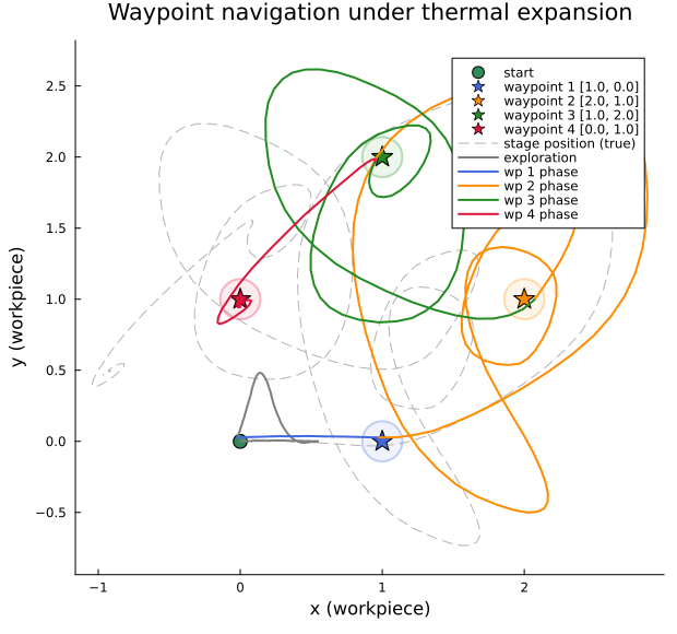

Thermal state and expansion offset

The upper panel shows the thermal state $T_k$ (hidden from the agent) together with the steady-state value $T_\infty = \eta P / \kappa$. The lower panel shows the magnitude of the thermal offset $\|\alpha(T_k - T_\text{amb})\|$ that the agent's observations carry. Vertical dashed lines mark goal switches.

t_axis   = Δt .* (1:len_trial)
T_steady = stage.eta * stage.P_proc / stage.kappa
alpha_v  = stage.alpha
offset   = [norm(alpha_v .* T_sim[k]) for k in 1:len_trial]

pT = plot(t_axis, T_sim, label="T (true, hidden)", color="firebrick", linewidth=2)
hline!([T_steady], label="T∞ = $(T_steady)", linestyle=:dash, color="firebrick", alpha=0.5)
vline!([Δt .* goal_switches], linestyle=:dash, color="black", alpha=0.4, label="")
ylabel!("thermal state"); xlabel!("")

pO = plot(t_axis, offset, label="|α(T − T₀)|", color="darkorange", linewidth=2,
          xlabel="time (s)", ylabel="offset magnitude")
vline!([Δt .* goal_switches], linestyle=:dash, color="black", alpha=0.4, label="")

plot(pT, pO, layout=(2,1), size=(700, 420), legend=:right)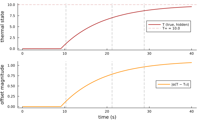

The expected free energy landscape

Evaluating $G(u)$ over the force space at a selected planning step reveals what the agent is optimising. The white marker is the chosen action.

function efe_landscape(u; tpoint, g)
    M = Ms[:, :, tpoint]; U = Us[:, :, tpoint]; V = Vs[:, :, tpoint]; ν = νs[tpoint]
    x = [y_sim[:, tpoint-1]; y_sim[:, tpoint-2]; u; u_sim[:, tpoint-1]; u_sim[:, tpoint-2]]
    η, μ, Σ = posterior_predictive(x, M, U, V, ν, Dx, Dy)
    return mutualinfo(Σ) + crossentropy(g, η, μ, Σ)
end

tp    = isempty(goal_switches) ? n_explore + 30 : goal_switches[1] + 20
g_tp  = MvNormalMeanCovariance(waypoints[wp_history[tp]], S_star)
ur    = range(u_lims[1], u_lims[2], length=61)
Gland = [efe_landscape([ui, uj], tpoint=tp, g=g_tp) for ui in ur, uj in ur]
gmin  = argmin(Gland)
pefe  = heatmap(ur, ur, Gland', color=:viridis,
                xlabel="force x (u₁)", ylabel="force y (u₂)",
                title="Expected free energy at step $tp", size=(560, 480))
scatter!([ur[gmin[1]]], [ur[gmin[2]]], color=:white, markersize=8, label="argmin")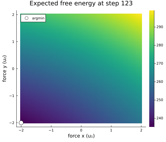

Animation

The animation shows the closed-loop behaviour: workpiece-frame trajectory (solid), true stage position (dashed), the active waypoint (bright star), and the one-step-ahead predictive belief (purple ellipse).

anim = @animate for k in 1:2:len_trial
    gi = wp_history[k]
    scatter([0.0], [0.0], color="seagreen", markersize=5, label="start",
            title="step $k / $len_trial  |  T=$(round(T_sim[k],digits=2))")
    for (i, w) in enumerate(waypoints)
        active = (i == gi)
        col    = wp_colors[i]
        scatter!([w[1]], [w[2]], marker=active ? :star8 : :star5, color=col,
                 markersize=active ? 12 : 7, alpha=active ? 1.0 : 0.4, label="")
        covellipse!(w, 5e-3 * diagm(ones(2)), n_std=2, linecolor=col,
                    color=col, fillalpha=active ? 0.12 : 0.03, linewidth=active ? 2 : 1, label="")
    end
    plot!(z_sim[1, 1:k], z_sim[2, 1:k], color="gray", linestyle=:dash,
          linewidth=1, alpha=0.5, label="stage (true)")
    plot!(y_sim[1, 1:k], y_sim[2, 1:k], color="royalblue", linewidth=2, label="workpiece (obs)")
    scatter!([y_sim[1, k]], [y_sim[2, k]], color="royalblue", markersize=5, label="")
    covellipse!(preds_m[:, k+1], preds_S[:, :, k+1], n_std=1,
                color="purple", fillalpha=0.15, label="prediction")
    plot!(xlims=(-1.5, 3.5), ylims=(-1.5, 3.5), aspect_ratio=:equal,
          legend=:topleft, size=(520, 520))
end
gif(anim, "thermal-stage-active-inference.gif", fps=12)

Plots.AnimatedGif("/home/runner/work/RxInferExamples.jl/RxInferExamples.jl/
docs/src/categories/advanced_examples/autoregressive_active_inference/therm
al-stage-active-inference.gif")

References

[1] Kouw, W. M., Nisslbeck, T. N., & Nuijten, W. L. N. (2026). Message Passing-Based Inference in an Autoregressive Active Inference Agent. In: Active Inference (IWAI 2025). Communications in Computer and Information Science, vol 2857, pp. 285–298. Springer, Cham. https://doi.org/10.1007/978-3-032-16955-6_16

Contributing

This example was automatically generated from a Jupyter notebook in the RxInferExamples.jl repository.

We welcome and encourage contributions! You can help by:

Improving this example
Creating new examples
Reporting issues or bugs
Suggesting enhancements

Visit our GitHub repository to get started. Together we can make RxInfer.jl even better! 💪

Environment

This example was executed in a clean, isolated environment. Below are the exact package versions used:

For reproducibility:

Use the same package versions when running locally
Report any issues with package compatibility

Status `/tmp/jl_CRjqkx/Project.toml`
  [b4ee3484] BayesBase v1.5.9
  [31c24e10] Distributions v0.25.129
⌅ [5b8099bc] DomainSets v0.7.18
  [62312e5e] ExponentialFamily v2.5.1
  [2d5283b6] FastCholesky v1.4.3
⌅ [f6369f11] ForwardDiff v0.10.39
  [429524aa] Optim v2.2.1
  [91a5bcdd] Plots v1.41.6
  [86711068] RxInfer v5.5.0
  [276daf66] SpecialFunctions v2.8.0
⌅ [4c63d2b9] StatsFuns v1.5.2
  [f3b207a7] StatsPlots v0.15.8
  [37e2e46d] LinearAlgebra v1.12.0
  [9a3f8284] Random v1.11.0
Info Packages marked with ⌅ have new versions available but compatibility constraints restrict them from upgrading. To see why use `status --outdated`