This example was automatically generated from a Jupyter notebook in the RxInferExamples.jl repository.
We welcome and encourage contributions! You can help by:
- Improving this example
- Creating new examples
- Reporting issues or bugs
- Suggesting enhancements
Visit our GitHub repository to get started. Together we can make RxInfer.jl even better! 💪
Contextual Bandits
We will start this notebook with a motivating example.
Let’s face it—ads are annoying. But very often they’re also one of the few ways to keep the business running. Imagine a free-to-play game for example. The real question isn’t whether to show ads, but when and which kind to show, so that players don’t feel bombarded, leave the game frustrated, or stop spending altogether.
It’s a balancing act between monetization and player retention.
If you show ads too aggressively, players quit. If you show ads too cautiously, you leave money on the table. So, how do you decide what to do in each moment of a player’s session?
Turning Ad Scheduling Into a Learning Problem
Every player session is different. Some players are engaged, some are rushing through, some just made a purchase, some are one level away from quitting.
At every possible ad moment, you have choices like:
- Show a video ad (high revenue, high interruption)
- Show a banner ad (low revenue, low interruption)
- Show no ad (defer to later)
And you have context—information about the session so far:
- Player’s level and progress
- Time since the last ad
- Time spent in the current session
- Whether the player just succeeded or failed at something
- Recent purchases or reward claims
What you want is a system that learns from player behavior over time, figuring out which actions perform best in which contexts—not just maximizing clicks or ad revenue right now, but balancing that with keeping players happy and playing longer.
Contextual Multi-Armed Bandits to the Rescue
This is exactly where Contextual Multi-Armed Bandits (CMABs) come in.
Contextual Multi‑Armed Bandits (CMABs) extend the classic bandit setting by allowing the learner to observe a context—a feature vector that describes the current situation—before selecting an action (or arm). The learner’s aim is to maximise cumulative reward over time by repeatedly balancing:
- Exploration – trying arms whose pay‑offs are still uncertain in some contexts.
- Exploitation – choosing the arm with the highest estimated reward in the current context.
CMABs sit between simple A/B tests and full reinforcement‑learning problems and are the work‑horse behind many personalisation engines.
Acting identically for every context wastes opportunity; CMABs formalise how to adapt decisions on‑the‑fly.
Implementing CMABs in RxInfer.jl
In this notebook we will implement a CMAB in RxInfer.jl way. A way to tackle CMAB in RxInfer requires expressing the generative model as a hierarchical Bayesian linear‑regression model and then message passing inference will do the rest.
Generative model (consistent notation)
Let
\[K\]
– number of arms.\[d\]
– dimension of the context vector.\[c_t\in\mathbb{R}^d\]
– context observed at round $t$.\[a_t\in{1,\dots,K}\]
– arm selected at round $t$.\[r_t\in\mathbb{R}\]
– realised reward.
The environment produces rewards according to:
- Global noise precision $\tau\;\sim\;\mathcal{G}(\alpha_\tau, \beta_\tau)$
- Arm‑specific regression parameters $k = 1,\dots,K$ $\theta_k \;\sim\; \mathcal{N}(m_{0k}, V_{0k}), \qquad \\ \Lambda_k \;\sim\; \operatorname{Wishart}(\nu_{0k}, W_{0k})$
- Per interaction latent coefficients $t = 1,\dots,T$ $\beta_t \;\sim\; \mathcal{N}(\theta_{a_t}, \Lambda_{a_t}^{-1})$
- Reward generation $\mu_t = c_t^\top \beta_t, \qquad \\ r_t \;\sim\; \mathcal{N}(\mu_t, \tau^{-1})$
Interpretation. Each arm owns a distribution of weight vectors ($\theta_k$), capturing how the context maps to reward for that arm. On every play we draw a concrete weight vector $\beta_t$, compute the expected reward $\mu_t$, and then observe a noisy realisation $r_t$.
Inference & decision‑making
With RxInfer we:
- Declare the model above with the
@modelmacro. (To make the example simpler, we'll have two models: one for parameters and one for predictions. A more complex scenario would be to have a single model for both.) - Stream incoming tuples $(c_t, a_t, r_t)$.
- Call
inferto update the posterior over $(\theta_k, \Lambda_k, \tau)$. - Compute predictive distributions of rewards in a new context $c_{t+1}$ via
inferon the predictive model: - Choose the next arm based on sampled from the predictive distribution.
Because both learning and prediction are expressed as probabilistic inference, we keep all uncertainty in closed form—ideal for principled exploration. The same pipeline generalises easily to non‑linear contexts (via feature maps) or non‑Gaussian rewards by swapping likelihood terms.
using RxInfer, Distributions, LinearAlgebra, Plots, StatsPlots, ProgressMeter, StableRNGs, RandomAt first let's generate synthetic data to simulate the CMAB problem.
using StableRNGs

# Random number generator
rng = StableRNG(42)

# Data generation parameters
n_train_samples = 300
n_test_samples = 100
n_total_samples = n_train_samples + n_test_samples
n_arms = 10
n_contexts = 50
context_dim = 20
noise_sd = 0.1

# Generate true arm parameters (θ_k in the model description)
arms = [randn(rng, context_dim) for _ in 1:n_arms]

# Generate context feature vectors with missing values
contexts = []
for i in 1:n_contexts
    # Create a vector that can hold both Float64 and Missing values
    context = Vector{Union{Float64,Missing}}(undef, context_dim)

    # Fill with random values initially
    for j in 1:context_dim
        context[j] = randn(rng)
    end

    # Randomly introduce missing values in some contexts
    if rand(rng) < 0.4  # 40% of contexts will have some missing values
        n_missing = rand(rng, 1:2)  # 1-2 missing values per context

        # Simple approach: randomly select indices for missing values
        missing_indices = []
        while length(missing_indices) < n_missing
            idx = rand(rng, 1:context_dim)
            if !(idx in missing_indices)
                push!(missing_indices, idx)
            end
        end

        for idx in missing_indices
            context[idx] = missing
        end
    end

    push!(contexts, context)
end

# Synthetic reward function (reusable)
function compute_reward(arm_params, context_vec, noise_sd=0.0; rng=nothing)
    """
    Compute reward for given arm parameters and context.

    Args:
        arm_params: Vector of arm parameters
        context_vec: Context vector (may contain missing values)
        noise_sd: Standard deviation of Gaussian noise to add
        rng: Random number generator (optional, for reproducible noise)

    Returns:
        Scalar reward value
    """
    # Calculate the deterministic part of the reward, handling missing values
    mean_reward = 0.0
    valid_dims = 0

    for j in 1:length(context_vec)
        if !ismissing(context_vec[j])
            mean_reward += arm_params[j] * context_vec[j]
            valid_dims += 1
        end
    end

    # Normalize by the number of valid dimensions to maintain similar scale
    if valid_dims > 0
        mean_reward = mean_reward * (length(context_vec) / valid_dims)
    end

    # Add Gaussian noise if requested
    if noise_sd > 0
        if rng !== nothing
            mean_reward += randn(rng) * noise_sd
        else
            mean_reward += randn() * noise_sd
        end
    end

    return mean_reward
end

# Generate training and test data
function generate_bandit_data(n_samples, arms, contexts, noise_sd; rng, start_idx=1)
    """
    Generate bandit data for given number of samples.

    Returns:
        (arm_choices, context_choices, rewards)
    """
    arm_choices = []
    context_choices = []
    rewards = []

    for i in 1:n_samples
        # Randomly select a context and an arm
        push!(context_choices, rand(rng, 1:length(contexts)))
        push!(arm_choices, rand(rng, 1:length(arms)))

        # Get the selected context and arm
        selected_context = contexts[context_choices[end]]
        selected_arm = arms[arm_choices[end]]

        # Compute reward using the synthetic reward function
        reward = compute_reward(selected_arm, selected_context, noise_sd; rng=rng)
        push!(rewards, reward)
    end

    return arm_choices, context_choices, rewards
end

# Generate training data
println("Generating training data...")
train_arm_choices, train_context_choices, train_rewards = generate_bandit_data(
    n_train_samples, arms, contexts, noise_sd; rng=rng
)

# Generate test data
println("Generating test data...")
test_arm_choices, test_context_choices, test_rewards = generate_bandit_data(
    n_test_samples, arms, contexts, noise_sd; rng=rng
)

# Display information about the generated data
println("\nDataset Summary:")
println("Training samples: $n_train_samples")
println("Test samples: $n_test_samples")
println("Total contexts: $(length(contexts))")
println("Number of contexts with missing values: ", sum(any(ismissing, ctx) for ctx in contexts))
println("Arms: $n_arms")
println("Context dimension: $context_dim")
println("Noise standard deviation: $noise_sd")

# Show examples of contexts with missing values
println("\nExamples of contexts with missing values:")
count = 0
for (i, ctx) in enumerate(contexts)
    if any(ismissing, ctx) && count < 3  # Show first 3 examples
        println("Context $i: $ctx")
        global count += 1
    end
end

# Show sample data
println("\nTraining data samples (first 5):")
for i in 1:min(5, length(train_rewards))
    println("Sample $i: Arm=$(train_arm_choices[i]), Context=$(train_context_choices[i]), Reward=$(round(train_rewards[i], digits=4))")
end

println("\nTest data samples (first 5):")
for i in 1:min(5, length(test_rewards))
    println("Sample $i: Arm=$(test_arm_choices[i]), Context=$(test_context_choices[i]), Reward=$(round(test_rewards[i], digits=4))")
end

# Verify the reward function works correctly
println("\nTesting reward function:")
test_context = contexts[1]
test_arm = arms[1]
deterministic_reward = compute_reward(test_arm, test_context, 0.0)  # No noise
noisy_reward = compute_reward(test_arm, test_context, noise_sd; rng=rng)  # With noise
println("Deterministic reward: $(round(deterministic_reward, digits=4))")
println("Noisy reward: $(round(noisy_reward, digits=4))")
Generating training data...
Generating test data...
Dataset Summary:
Training samples: 300
Test samples: 100
Total contexts: 50
Number of contexts with missing values: 22
Arms: 10
Context dimension: 20
Noise standard deviation: 0.1
Examples of contexts with missing values:
Context 3: Union{Missing, Float64}[missing, -0.4741385118651381, -1.0989041
9081401, -1.079288892379018, 0.8184199040107111, -0.30409464242950546, -0.6
709508997562322, -0.7469592378369052, 0.21407501633089995, -0.6139813001136
504, 2.8170273653049507, -1.4362435690909499, -0.30112508107598307, -0.3868
83090487843, 0.6563571763621648, 1.401591444397142, 0.6193863742347839, 0.1
2760715013378465, -0.2758495479700435, 1.8822768045661076]
Context 8: Union{Missing, Float64}[-2.3650237776747054, -1.1739461025984783
, 1.128284045692684, -0.8690689832066373, 0.4497591893001418, -0.2617237965
612964, 0.07868265261314639, missing, 1.9119126287271901, 0.719828217704402
8, -2.708690227134825, -2.645555311022844, -0.3202946667428825, 1.398258591
17344, 0.06974735851443013, 1.1639494445584129, -0.36687387238833036, 0.506
2972107773495, -1.3675557327045547, missing]
Context 9: Union{Missing, Float64}[-0.7928407885849085, 0.5230893424666117,
0.21944291871653826, -0.2951043978830045, missing, 0.6739591611416778, 0.6
091981160535558, 0.37661376790321904, -0.08201072963796563, 0.6762611326141
408, -1.7998621684347569, 0.7079334064897562, -1.5082653360123872, 0.423324
15672698104, 1.380447484940245, -3.325041477189219, 1.1893655835458625, 0.9
25128468276957, -1.62673585658528, -0.667629748025382]
Training data samples (first 5):
Sample 1: Arm=6, Context=11, Reward=2.7556
Sample 2: Arm=2, Context=14, Reward=-3.911
Sample 3: Arm=8, Context=14, Reward=-2.0472
Sample 4: Arm=6, Context=36, Reward=9.6666
Sample 5: Arm=3, Context=21, Reward=-4.1496
Test data samples (first 5):
Sample 1: Arm=1, Context=18, Reward=0.3271
Sample 2: Arm=2, Context=27, Reward=-3.2327
Sample 3: Arm=4, Context=4, Reward=-2.1027
Sample 4: Arm=1, Context=7, Reward=4.7518
Sample 5: Arm=8, Context=24, Reward=3.4953
Testing reward function:
Deterministic reward: -2.2755
Noisy reward: -2.2613function create_bandit_plots(arm_choices, context_choices, rewards, title_prefix, color_scheme)
p1 = scatter(1:length(context_choices), context_choices,
label="Context Choices",
title="$title_prefix: Context Selection",
xlabel="Sample", ylabel="Context ID",
marker=:circle, markersize=6,
color=color_scheme[:context], alpha=0.7)
p2 = scatter(1:length(arm_choices), arm_choices,
label="Arm Choices",
title="$title_prefix: Arm Selection",
xlabel="Sample", ylabel="Arm ID",
marker=:diamond, markersize=6,
color=color_scheme[:arm], alpha=0.7)
p3 = plot(1:length(rewards), rewards,
label="Rewards",
title="$title_prefix: Rewards",
xlabel="Sample", ylabel="Reward Value",
linewidth=2, marker=:star, markersize=4,
color=color_scheme[:reward], alpha=0.8)
hline!(p3, [mean(rewards)], label="Mean Reward",
linestyle=:dash, linewidth=2, color=:black)
return plot(p1, p2, p3, layout=(3, 1), size=(800, 600))
end
# Create training plots
train_colors = Dict(:context => :blue, :arm => :red, :reward => :green)
train_plot = create_bandit_plots(train_arm_choices, train_context_choices, train_rewards,
"Training Data", train_colors)
# Create test plots
test_colors = Dict(:context => :lightblue, :arm => :pink, :reward => :lightgreen)
test_plot = create_bandit_plots(test_arm_choices, test_context_choices, test_rewards,
"Test Data", test_colors)
# Display both
plot(train_plot, test_plot, layout=(1, 2), size=(1600, 600),
plot_title="Contextual Bandit Experiment: Training and Test Data")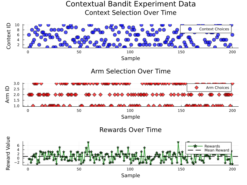
@model function conditional_regression(n_arms, priors, past_rewards, past_choices, past_contexts)
    local θ
    local γ
    local τ

    # Prior for each arm's parameters
    for k in 1:n_arms
        θ[k] ~ priors[:θ][k]
        γ[k] ~ priors[:γ][k]
    end

    # Prior for the noise precision
    τ ~ priors[:τ]

    # Model for past observations
    for n in eachindex(past_rewards)
        arm_vals[n] ~ NormalMixture(switch=past_choices[n], m=θ, p=γ)
        latent_context[n] ~ past_contexts[n]
        past_rewards[n] ~ softdot(arm_vals[n], latent_context[n], τ)
    end
end
Let's define the priors.
priors_rng = StableRNG(42)
priors = Dict(
    :θ => [MvNormalMeanPrecision(randn(priors_rng, context_dim), diagm(ones(context_dim))) for _ in 1:n_arms],
    :γ => [Wishart(context_dim + 1, diagm(ones(context_dim))) for _ in 1:n_arms],
    :τ => GammaShapeRate(1.0, 1.0)
)
Dict{Symbol, Any} with 3 entries:
:γ => Wishart{Float64, PDMat{Float64, Matrix{Float64}}, Int64}[Distributi
ons.…
:τ => ExponentialFamily.GammaShapeRate{Float64}(a=1.0, b=1.0)
:θ => MvNormalMeanPrecision{Float64, Vector{Float64}, Matrix{Float64}}[Mv
Norm…And finally run the inference.
function run_inference(; n_arms, priors, past_rewards, past_choices, past_contexts, iterations=50, free_energy=true)
    init = @initialization begin
        q(θ) = priors[:θ]
        q(γ) = priors[:γ]
        q(τ) = priors[:τ]
        q(latent_context) = MvNormalMeanPrecision(zeros(context_dim), Diagonal(ones(context_dim)))
    end

    return infer(
        model=conditional_regression(
            n_arms=n_arms,
            priors=priors,
            past_contexts=past_contexts,
        ),
        data=(
            past_rewards=past_rewards,
            past_choices=past_choices,
        ),
        constraints=MeanField(),
        initialization=init,
        showprogress=true,
        iterations=iterations,
        free_energy=free_energy
    )

end
run_inference (generic function with 1 method)# Utility function to convert context with missing values to MvNormal distribution
function context_to_mvnormal(context_vec; tiny_precision=1e-6, huge_precision=1e6)
"""
Convert a context vector (potentially with missing values) to MvNormal distribution.
Args:
context_vec: Vector that may contain missing values
tiny_v: Small variance for known values (high precision)
huge_var: Large variance for missing values (low precision)
Returns:
MvNormal distribution
"""
context_mean = Vector{Float64}(undef, length(context_vec))
context_precision = Vector{Float64}(undef, length(context_vec))
for j in 1:length(context_vec)
if ismissing(context_vec[j])
context_mean[j] = 0.0
context_precision[j] = tiny_precision
else
context_mean[j] = context_vec[j]
context_precision[j] = huge_precision
end
end
return MvNormalMeanPrecision(context_mean, Diagonal(context_precision))
endcontext_to_mvnormal (generic function with 1 method)# Convert to the required types for the model (TRAINING DATA ONLY)
rewards_data = Float64.(train_rewards)
# Parameters for the covariance matrix
tiny_precision = 1e-6 # Very high precision (small variance) for known values
huge_precision = 1e6 # Very low precision (large variance) for missing values
contexts_data = [
let context = contexts[idx]
context_to_mvnormal(context; tiny_precision=tiny_precision, huge_precision=huge_precision)
end
for idx in train_context_choices # Use training context choices
]
arm_choices_data = [[Float64(k == chosen_arm) for k in 1:n_arms] for chosen_arm in train_arm_choices]; # Use training arm choicesresult = run_inference(
n_arms=n_arms,
priors=priors,
past_rewards=rewards_data,
past_choices=arm_choices_data,
past_contexts=contexts_data,
iterations=20,
free_energy=false
)Inference results:
Posteriors | available for (γ, arm_vals, τ, latent_context, θ)# Diagnostics of inferred arms
# 1. MSE of inferred arms coefficients
inferred_arms = mean.(result.posteriors[:θ][end])
mse_arms = mean(mean((inferred_arms[i] .- arms[i]) .^ 2) for i in eachindex(arms))
println("MSE of inferred arm coefficients: $mse_arms")MSE of inferred arm coefficients: 0.005138753286482585# Function to compute predicted rewards using softdot rules
function compute_predicted_rewards_with_variance(
arm_posteriors,
precision_posterior,
eval_arm_choices,
eval_context_choices,
eval_rewards
)
predicted_rewards = []
reward_variances = []
for i in 1:length(eval_rewards) # Evaluate on all samples in the evaluation set
arm_idx = eval_arm_choices[i]
ctx_idx = eval_context_choices[i]
# Get the posterior distributions
q_arm = arm_posteriors[arm_idx] # Posterior over arm parameters
q_precision = precision_posterior # Precision posterior
# Get the actual context and convert to MvNormal
actual_context = contexts[ctx_idx]
q_context = context_to_mvnormal(actual_context)
# Use softdot rule to compute predicted reward distribution
predicted_reward_dist = NormalMeanPrecision(
mean(q_arm)' * mean(q_context),
mean(q_precision)
)
push!(predicted_rewards, mean(predicted_reward_dist))
push!(reward_variances, var(predicted_reward_dist))
end
return predicted_rewards, reward_variances
end
# Function to display evaluation results
function display_evaluation_results(predicted_rewards, reward_variances, actual_rewards,
arm_choices, context_choices, dataset_name)
println("\n$dataset_name Evaluation Results:")
println("Sample | Actual Reward | Predicted Mean | Predicted Std | Arm | Context")
println("-------|---------------|----------------|---------------|-----|--------")
for i in 1:min(10, length(predicted_rewards))
actual = actual_rewards[i]
pred_mean = predicted_rewards[i]
pred_std = sqrt(reward_variances[i])
arm_idx = arm_choices[i]
ctx_idx = context_choices[i]
println("$(lpad(i, 6)) | $(rpad(round(actual, digits=4), 13)) | $(rpad(round(pred_mean, digits=4), 14)) | $(rpad(round(pred_std, digits=4), 13)) | $(lpad(arm_idx, 3)) | $(lpad(ctx_idx, 7))")
end
# Compute prediction metrics
prediction_mse = mean((predicted_rewards .- actual_rewards) .^ 2)
println("\n$dataset_name Prediction MSE: $prediction_mse")
# Compute log-likelihood of actual rewards under predicted distributions
log_likelihood = sum(
logpdf(Normal(predicted_rewards[i], sqrt(reward_variances[i])), actual_rewards[i])
for i in 1:length(predicted_rewards)
)
println("$dataset_name Average log-likelihood: $(log_likelihood / length(predicted_rewards))")
return prediction_mse, log_likelihood / length(predicted_rewards)
end
# Evaluate on TRAINING data
println("=== TRAINING DATA EVALUATION ===")
train_predicted_rewards, train_reward_variances = compute_predicted_rewards_with_variance(
result.posteriors[:θ][end], # Use full posteriors
result.posteriors[:τ][end], # Precision posterior
train_arm_choices,
train_context_choices,
train_rewards
)
train_mse, train_ll = display_evaluation_results(
train_predicted_rewards,
train_reward_variances,
train_rewards,
train_arm_choices,
train_context_choices,
"Training"
)
# Evaluate on TEST data
println("\n=== TEST DATA EVALUATION ===")
test_predicted_rewards, test_reward_variances = compute_predicted_rewards_with_variance(
result.posteriors[:θ][end], # Use full posteriors
result.posteriors[:τ][end], # Precision posterior
test_arm_choices,
test_context_choices,
test_rewards
)
test_mse, test_ll = display_evaluation_results(
test_predicted_rewards,
test_reward_variances,
test_rewards,
test_arm_choices,
test_context_choices,
"Test"
)
# Summary comparison
println("\n=== SUMMARY COMPARISON ===")
println("Dataset | MSE | Log-Likelihood")
println("-----------|----------|---------------")
println("Training | $(rpad(round(train_mse, digits=4), 8)) | $(round(train_ll, digits=4))")
println("Test | $(rpad(round(test_mse, digits=4), 8)) | $(round(test_ll, digits=4))")
if test_mse > train_mse * 1.2
println("\nNote: Test MSE is significantly higher than training MSE - possible overfitting")
elseif test_mse < train_mse * 0.8
println("\nNote: Test MSE is lower than training MSE - good generalization!")
else
println("\nNote: Test and training performance are similar - good generalization")
end=== TRAINING DATA EVALUATION ===
Training Evaluation Results:
Sample | Actual Reward | Predicted Mean | Predicted Std | Arm | Context
-------|---------------|----------------|---------------|-----|--------
1 | 2.7556 | 2.7721 | 1.3082 | 6 | 11
2 | -3.911 | -3.535 | 1.3082 | 2 | 14
3 | -2.0472 | -1.8887 | 1.3082 | 8 | 14
4 | 9.6666 | 8.1026 | 1.3082 | 6 | 36
5 | -4.1496 | -3.8266 | 1.3082 | 3 | 21
6 | -4.7496 | -4.5237 | 1.3082 | 4 | 49
7 | -2.1116 | -2.1877 | 1.3082 | 5 | 34
8 | 0.3173 | 0.5183 | 1.3082 | 8 | 32
9 | -4.9155 | -4.1394 | 1.3082 | 8 | 49
10 | -3.0535 | -3.3429 | 1.3082 | 6 | 31
Training Prediction MSE: 0.16609598579011065
Training Average log-likelihood: -1.236149219320253
=== TEST DATA EVALUATION ===
Test Evaluation Results:
Sample | Actual Reward | Predicted Mean | Predicted Std | Arm | Context
-------|---------------|----------------|---------------|-----|--------
1 | 0.3271 | 0.0431 | 1.3082 | 1 | 18
2 | -3.2327 | -2.6156 | 1.3082 | 2 | 27
3 | -2.1027 | -1.8232 | 1.3082 | 4 | 4
4 | 4.7518 | 4.465 | 1.3082 | 1 | 7
5 | 3.4953 | 2.9212 | 1.3082 | 8 | 24
6 | 1.0455 | 0.3028 | 1.3082 | 4 | 15
7 | -0.2608 | -0.2963 | 1.3082 | 9 | 38
8 | -6.0007 | -5.6078 | 1.3082 | 8 | 1
9 | -3.1662 | -2.8644 | 1.3082 | 7 | 36
10 | 0.9946 | 1.1453 | 1.3082 | 10 | 24
Test Prediction MSE: 0.17808283508293526
Test Average log-likelihood: -1.2396510580518532
=== SUMMARY COMPARISON ===
Dataset | MSE | Log-Likelihood
-----------|----------|---------------
Training | 0.1661 | -1.2361
Test | 0.1781 | -1.2397
Note: Test and training performance are similar - good generalization# Additional diagnostics
println("\n=== ADDITIONAL DIAGNOSTICS ===")
# Show precision/variance information
precision_posterior = result.posteriors[:τ][end]
println("Inferred noise precision: mean=$(round(mean(precision_posterior), digits=4)), " *
"std=$(round(std(precision_posterior), digits=4))")
println("Inferred noise variance: $(round(1/mean(precision_posterior), digits=4))")
println("True noise variance: $(round(noise_sd^2, digits=4))")
# Show arm coefficient statistics
println("\nArm coefficient comparison:")
for i in eachindex(arms)
true_arm = arms[i]
inferred_arm_posterior = result.posteriors[:θ][end][i]
inferred_arm_mean = mean(inferred_arm_posterior)
println("Arm $i:")
println(" True: $(round.(true_arm, digits=3))")
println(" Inferred: $(round.(inferred_arm_mean, digits=3))")
println(" MSE: $(round(mean((inferred_arm_mean .- true_arm).^2), digits=4))")
end
println("\nNumber of contexts with missing values: ", sum(any(ismissing, ctx) for ctx in contexts))=== ADDITIONAL DIAGNOSTICS ===
Inferred noise precision: mean=0.5843, std=0.0475
Inferred noise variance: 1.7115
True noise variance: 0.01
Arm coefficient comparison:
Arm 1:
True: [-0.67, 0.447, 1.374, 1.31, 0.126, 0.684, -1.019, -0.794, 1.775
, 1.297, -1.644, 0.794, -1.31, -0.037, 1.072, -0.397, -0.239, -0.651, 1.134
, -0.84]
Inferred: [-0.604, 0.429, 1.306, 1.212, 0.094, 0.665, -0.972, -0.744, 1.6
85, 1.264, -1.578, 0.765, -1.279, -0.01, 1.043, -0.381, -0.209, -0.582, 1.0
56, -0.76]
MSE: 0.003
Arm 2:
True: [2.085, -1.801, 0.483, -0.57, -0.665, 2.243, -1.464, -1.012, -2
.042, -0.787, 0.591, 0.642, 0.455, 0.054, 0.288, 0.587, -1.694, -0.696, -0.
301, 2.101]
Inferred: [1.997, -1.708, 0.451, -0.542, -0.636, 2.161, -1.364, -0.965, -
1.964, -0.754, 0.49, 0.614, 0.459, 0.044, 0.171, 0.557, -1.624, -0.59, -0.1
67, 2.001]
MSE: 0.0057
Arm 3:
True: [-0.69, -0.73, -1.417, -1.383, 1.201, 0.576, -0.987, 0.626, 0.1
87, 0.239, -1.287, 0.147, -0.345, 1.909, 0.093, -0.643, 0.743, 0.725, 0.077
, -0.008]
Inferred: [-0.655, -0.724, -1.353, -1.319, 1.132, 0.548, -0.898, 0.526, 0
.194, 0.232, -1.263, 0.115, -0.257, 1.834, 0.068, -0.568, 0.703, 0.694, 0.0
66, 0.001]
MSE: 0.0029
Arm 4:
True: [-0.37, 0.888, -1.056, 1.242, 0.628, 1.161, -0.851, -0.428, 0.1
09, -1.932, 0.105, 0.016, 0.105, 1.434, 0.141, 1.295, -0.931, 1.076, -1.799
, -0.822]
Inferred: [-0.23, 0.849, -1.04, 1.172, 0.477, 1.134, -0.779, -0.355, 0.12
8, -1.876, 0.097, 0.068, 0.037, 1.372, 0.124, 1.243, -0.905, 1.014, -1.727,
-0.796]
MSE: 0.0044
Arm 5:
True: [-0.217, 0.641, -1.566, -1.487, -0.45, -0.937, -0.59, 1.572, -0
.229, 0.473, 2.148, -0.614, -0.451, -1.672, -0.224, 0.461, -0.093, 1.038, -
1.827, 0.698]
Inferred: [-0.201, 0.628, -1.515, -1.422, -0.373, -0.907, -0.495, 1.468,
-0.22, 0.476, 2.079, -0.564, -0.238, -1.613, -0.101, 0.433, -0.104, 0.973,
-1.731, 0.634]
MSE: 0.0062
Arm 6:
True: [0.403, 0.333, 1.549, 0.156, 1.816, -0.626, -1.275, 0.485, 1.23
5, -1.121, -1.397, -0.658, -1.516, -0.712, -0.411, -1.254, 2.082, -0.53, -1
.64, -0.769]
Inferred: [0.227, 0.312, 1.496, 0.107, 1.705, -0.594, -1.151, 0.383, 1.17
4, -1.069, -1.351, -0.631, -1.445, -0.645, -0.4, -1.167, 2.001, -0.41, -1.5
89, -0.716]
MSE: 0.0064
Arm 7:
True: [1.528, 0.269, 1.215, 0.067, 0.84, 0.819, -1.459, 0.689, -1.067
, 1.278, -0.364, -1.031, -0.452, -1.973, 0.266, 0.212, -0.424, -1.286, 0.57
5, 0.72]
Inferred: [1.427, 0.271, 1.184, 0.041, 0.669, 0.79, -1.354, 0.645, -1.021
, 1.246, -0.335, -0.992, -0.375, -1.893, 0.271, 0.224, -0.355, -1.19, 0.552
, 0.696]
MSE: 0.0044
Arm 8:
True: [-0.651, -1.01, -0.863, 1.512, 0.743, -1.477, -0.288, -0.288, -
0.496, -0.151, 0.53, -0.429, -1.288, 0.95, 2.584, 0.719, -0.205, 1.232, -1.
135, -0.626]
Inferred: [-0.581, -0.964, -0.852, 1.411, 0.673, -1.425, -0.219, -0.262,
-0.466, -0.11, 0.486, -0.396, -1.228, 0.854, 2.469, 0.685, -0.191, 1.095, -
1.062, -0.546]
MSE: 0.0047
Arm 9:
True: [-1.049, 2.431, -0.434, 0.316, 1.271, -0.947, 0.131, 0.423, 0.1
62, -1.648, -0.058, -0.573, 1.01, -0.237, 0.212, -0.347, 0.143, -1.574, 0.7
96, 0.944]
Inferred: [-1.0, 2.341, -0.415, 0.143, 1.223, -0.91, 0.113, 0.439, 0.094,
-1.557, -0.066, -0.531, 0.986, -0.146, 0.122, -0.118, 0.131, -1.518, 0.769
, 0.869]
MSE: 0.0069
Arm 10:
True: [0.447, -1.369, 0.6, 0.392, -0.449, 0.049, -0.558, -1.213, -0.2
44, -0.289, 0.85, -0.834, 0.803, 1.531, -0.387, -1.258, -1.299, -1.05, -0.2
37, 0.536]
Inferred: [0.368, -1.322, 0.586, 0.295, -0.191, 0.04, -0.502, -1.155, -0.
24, -0.256, 0.813, -0.81, 0.782, 1.47, -0.29, -1.197, -1.278, -0.936, -0.14
6, 0.505]
MSE: 0.0067
Number of contexts with missing values: 22Comparing Different Strategies for the Contextual Bandit Problem
We'll implement and evaluate three different approaches:
- Random Strategy - Selecting arms randomly without using context information
- Vanilla Thompson Sampling - Sampling the reward distribution
- RxInfer Predictive Inference - Approximating the predictive posterior via message-passing
function random_strategy(; rng, n_arms)
    chosen_arm = rand(rng, 1:n_arms)
    return chosen_arm
end

function thompson_strategy(; rng, n_arms, current_context, posteriors)
    # Thompson Sampling: Sample parameter vectors and choose best arm
    expected_rewards = zeros(n_arms)
    for k in 1:n_arms
        # Sample parameters from posterior
        theta_sample = rand(rng, posteriors[:θ][k])
        # context might have missing values, so we use the mean of the context
        augmented_context = mean(context_to_mvnormal(current_context))
        expected_rewards[k] = dot(theta_sample, augmented_context)
    end

    # Choose best arm based on sampled parameters
    chosen_arm = argmax(expected_rewards)

    return chosen_arm
end
thompson_strategy (generic function with 1 method)@model function contextual_bandit_predictive(reward, priors, current_context)
local θ
local γ
local τ
# Prior for each arm's parameters
for k in 1:n_arms
θ[k] ~ priors[:θ][k]
γ[k] ~ priors[:γ][k]
end
τ ~ priors[:τ]
chosen_arm ~ Categorical(ones(n_arms) ./ n_arms)
arm_vals ~ NormalMixture(switch=chosen_arm, m=θ, p=γ)
latent_context ~ current_context
reward ~ softdot(arm_vals, latent_context, τ)
end
function predictive_strategy(; rng, n_arms, current_context, posteriors)
priors = Dict(
:θ => posteriors[:θ],
:γ => posteriors[:γ],
:τ => posteriors[:τ]
)
latent_context = context_to_mvnormal(current_context)
init = @initialization begin
q(θ) = priors[:θ]
q(τ) = priors[:τ]
q(γ) = priors[:γ]
q(latent_context) = latent_context
q(chosen_arm) = Categorical(ones(n_arms) ./ n_arms)
end
result = infer(
model=contextual_bandit_predictive(
priors=priors,
current_context=latent_context
),
data=(reward=10maximum(train_rewards),),
constraints=MeanField(),
initialization=init,
showprogress=true,
iterations=20,
)
chosen_arm = argmax(probvec(result.posteriors[:chosen_arm][end]))
return chosen_arm
endpredictive_strategy (generic function with 1 method)As we defined the strategies, we can proceed to defining the helper functions to run the simulation.
We will use the following flow:
- PLAN - Run different strategies
- ACT - In this simulation, we're evaluating all strategies in parallel
- OBSERVE - Get rewards for all strategies
- LEARN - Update posteriors based on history
- KEEP HISTORY - Record all results
# Helper functions
function select_context(rng, n_contexts)
    idx = rand(rng, 1:n_contexts)
    return (index=idx, value=contexts[idx])
end

function plan(rng, n_arms, context, posteriors)
    # Generate actions from different strategies
    return Dict(
        :random => random_strategy(rng=rng, n_arms=n_arms),
        :thompson => thompson_strategy(rng=rng, n_arms=n_arms, current_context=context, posteriors=posteriors),
        :predictive => predictive_strategy(rng=rng, n_arms=n_arms, current_context=context, posteriors=posteriors)
    )
end

function act(rng, strategies)
    # Here one would choose which strategy to actually follow
    # For this simulation, we're evaluating all in parallel
    # In a real scenario, one might return just one: return strategies[:thompson]
    return strategies
end

function observe(rng, strategies, context, arms, noise_sd)
    rewards = Dict()
    for (strategy, arm_idx) in strategies
        rewards[strategy] = compute_reward(arms[arm_idx], context, noise_sd)
    end
    return rewards
end

function learn(rng, n_arms, posteriors, past_rewards, past_choices, past_contexts)
    # Note that we don't do any forgetting here which might be useful for long-term learning
    # Prepare priors from current posteriors
    priors = Dict(:θ => posteriors[:θ], :τ => posteriors[:τ], :γ => posteriors[:γ])

    # Default initialization
    init = @initialization begin
        q(θ) = priors[:θ]
        q(τ) = priors[:τ]
        q(γ) = priors[:γ]
        q(latent_context) = MvNormalMeanPrecision(zeros(context_dim), Diagonal(ones(context_dim)))
    end

    # Run inference
    results = infer(
        model=conditional_regression(
            n_arms=n_arms,
            priors=priors,
            past_contexts=context_to_mvnormal.(past_contexts),
        ),
        data=(
            past_rewards=past_rewards,
            past_choices=past_choices,
        ),
        returnvars=KeepLast(),
        constraints=MeanField(),
        initialization=init,
        iterations=20,
        free_energy=false
    )

    return results.posteriors
end

function keep_history!(n_arms, history, strategies, rewards, context, posteriors)
    # Update choices
    for (strategy, arm_idx) in strategies
        push!(history[:choices][strategy], [Float64(k == arm_idx) for k in 1:n_arms])
    end

    # Update rewards
    for (strategy, reward) in rewards
        push!(history[:rewards][strategy], reward)
    end

    # Update real history - using predictive strategy as the actual choice
    push!(history[:real][:rewards], last(history[:rewards][:predictive]))
    push!(history[:real][:choices], last(history[:choices][:predictive]))

    # Update contexts
    push!(history[:contexts][:values], context.value)
    push!(history[:contexts][:indices], context.index)

    # Update posteriors
    push!(history[:posteriors], deepcopy(posteriors))
end
keep_history! (generic function with 1 method)function run_bandit_simulation(n_epochs, window_length, n_arms, n_contexts, context_dim)
rng = StableRNG(42)
# Initialize histories with empty arrays, removing the references to undefined variables
history = Dict(
:rewards => Dict(:random => [], :thompson => [], :predictive => []),
:choices => Dict(:random => [], :thompson => [], :predictive => []),
:real => Dict(:rewards => [], :choices => []),
:contexts => Dict(:values => [], :indices => []),
:posteriors => []
)
# Initialize prior posterior as uninformative
posteriors = Dict(:θ => [MvNormalMeanPrecision(randn(rng, context_dim), diagm(ones(context_dim))) for _ in 1:n_arms],
:γ => [Wishart(context_dim + 1, diagm(ones(context_dim))) for _ in 1:n_arms],
:τ => GammaShapeRate(1.0, 1.0))
@showprogress for epoch in 1:n_epochs
# 1. PLAN - Run different strategies
current_context = select_context(rng, n_contexts)
strategies = plan(rng, n_arms, current_context.value, posteriors)
# 2. ACT - In this simulation, we're evaluating all strategies in parallel
# In a real scenario, you might choose one strategy here
chosen_arm = act(rng, strategies)
# 3. OBSERVE - Get rewards for all strategies
rewards = observe(rng, strategies, current_context.value, arms, noise_sd)
# 4. LEARN - Update posteriors based on history
# Only try to learn if we have collected data
if mod(epoch, window_length) == 0 && length(history[:real][:rewards]) > 0
data_idx = max(1, length(history[:real][:rewards]) - window_length + 1):length(history[:real][:rewards])
posteriors = learn(
rng,
n_arms,
posteriors,
history[:real][:rewards][data_idx],
history[:real][:choices][data_idx],
history[:contexts][:values][data_idx]
)
end
# 5. KEEP HISTORY - Record all results
keep_history!(n_arms, history, strategies, rewards, current_context, posteriors)
end
return history
endrun_bandit_simulation (generic function with 1 method)# Run the simulation
n_epochs = 5000
window_length = 100
history = run_bandit_simulation(n_epochs, window_length, n_arms, n_contexts, context_dim)Dict{Symbol, Any} with 5 entries:
:choices => Dict{Symbol, Vector{Any}}(:predictive=>[[1.0, 0.0, 0.0, 0.
0, 0…
:contexts => Dict{Symbol, Vector{Any}}(:values=>[Union{Missing, Float64
}[0.…
:real => Dict{Symbol, Vector{Any}}(:choices=>[[1.0, 0.0, 0.0, 0.0,
0.0,…
:rewards => Dict{Symbol, Vector{Any}}(:predictive=>[-1.82844, 6.6928,
6.79…
:posteriors => Any[Dict{Symbol, Any}(:γ=>Wishart{Float64, PDMat{Float64,
Matr…function print_summary_statistics(history, n_epochs)
# Additional summary statistics
println("Random strategy cumulative reward: $(sum(history[:rewards][:random]))")
println("Thompson strategy cumulative reward: $(sum(history[:rewards][:thompson]))")
println("Predictive strategy cumulative reward: $(sum(history[:rewards][:predictive]))")
println("Results after $n_epochs epochs:")
println("Random strategy average reward: $(mean(history[:rewards][:random]))")
println("Thompson strategy average reward: $(mean(history[:rewards][:thompson]))")
println("Predictive strategy average reward: $(mean(history[:rewards][:predictive]))")
end
# Print the summary statistics
print_summary_statistics(history, n_epochs)Random strategy cumulative reward: -573.3395336377982
Thompson strategy cumulative reward: 27932.69808844848
Predictive strategy cumulative reward: 25893.770489345912
Results after 5000 epochs:
Random strategy average reward: -0.11466790672755965
Thompson strategy average reward: 5.586539617689696
Predictive strategy average reward: 5.178754097869183function plot_arm_distribution(history, n_arms)
# Extract choices
random_choices = history[:choices][:random]
thompson_choices = history[:choices][:thompson]
predictive_choices = history[:choices][:predictive]
# Convert to arm indices
random_arms = [argmax(choice) for choice in random_choices]
thompson_arms = [argmax(choice) for choice in thompson_choices]
predictive_arms = [argmax(choice) for choice in predictive_choices]
# Count frequencies
arm_counts_random = zeros(Int, n_arms)
arm_counts_thompson = zeros(Int, n_arms)
arm_counts_predictive = zeros(Int, n_arms)
for arm in random_arms
arm_counts_random[arm] += 1
end
for arm in thompson_arms
arm_counts_thompson[arm] += 1
end
for arm in predictive_arms
arm_counts_predictive[arm] += 1
end
# Create grouped bar plot
bar_plot = groupedbar(
1:n_arms,
[arm_counts_random arm_counts_thompson arm_counts_predictive],
title="Arm Selection Distribution",
xlabel="Arm Index",
ylabel="Selection Count",
bar_position=:dodge,
bar_width=0.8,
alpha=0.7,
legend=:topright,
labels=["Random" "Thompson" "Predictive"]
)
return bar_plot
end
# Plot arm distribution
arm_distribution_plot = plot_arm_distribution(history, 10)
display(arm_distribution_plot)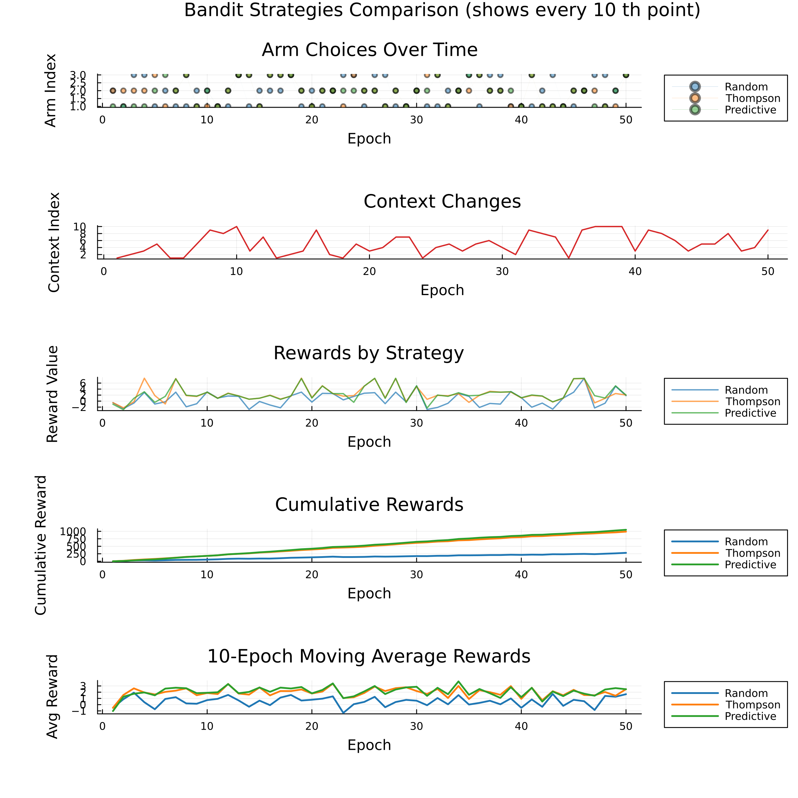
function calculate_improvements(history)
    # Get final average rewards
    final_random_avg = mean(history[:rewards][:random])
    final_thompson_avg = mean(history[:rewards][:thompson])
    final_predictive_avg = mean(history[:rewards][:predictive])

    # Improvements over random baseline
    thompson_improvement = (final_thompson_avg - final_random_avg) / abs(final_random_avg) * 100
    predictive_improvement = (final_predictive_avg - final_random_avg) / abs(final_random_avg) * 100

    println("Thompson sampling improves over random by $(round(thompson_improvement, digits=2))%")
    println("Predictive strategy improves over random by $(round(predictive_improvement, digits=2))%")

    return Dict(
        :thompson => thompson_improvement,
        :predictive => predictive_improvement
    )
end

# Calculate and display improvements
improvements = calculate_improvements(history)
Thompson sampling improves over random by 4971.93%
Predictive strategy improves over random by 4616.31%
Dict{Symbol, Float64} with 2 entries:
:predictive => 4616.31
:thompson => 4971.93function analyze_doubly_robust_uplift(history, target_strategy=:predictive, baseline_strategy=:random)
"""
Compute doubly robust uplift estimate from simulation history
"""
target_rewards = history[:rewards][target_strategy]
baseline_rewards = history[:rewards][baseline_strategy]
# Simple Direct Method - just difference in average rewards
direct_method = mean(target_rewards) - mean(baseline_rewards)
# For IPW, we use the fact that all strategies were evaluated on same contexts
# So propensity is uniform across arms for random, and we can estimate others
n_epochs = length(target_rewards)
n_arms = length(history[:choices][target_strategy][1])
# IPW correction (simplified since we have parallel evaluation)
ipw_correction = 0.0
for i in 1:n_epochs
# Get actual choice and reward (using predictive as "real" policy)
real_choice = history[:choices][:predictive][i]
real_reward = history[:rewards][:predictive][i]
target_choice = history[:choices][target_strategy][i]
baseline_choice = history[:choices][baseline_strategy][i]
# Simple propensity estimates
target_propensity = target_strategy == :random ? 1 / n_arms : 0.5 # rough estimate
baseline_propensity = baseline_strategy == :random ? 1 / n_arms : 0.5
# IPW terms (simplified)
if target_choice == real_choice
ipw_correction += real_reward / target_propensity
end
if baseline_choice == real_choice
ipw_correction -= real_reward / baseline_propensity
end
end
ipw_correction /= n_epochs
# Doubly robust = direct method + IPW correction
doubly_robust = direct_method + ipw_correction * 0.1 # damped correction
return Dict(
:direct_method => direct_method,
:doubly_robust => doubly_robust,
:target_mean => mean(target_rewards),
:baseline_mean => mean(baseline_rewards),
:uplift_percent => (direct_method / mean(baseline_rewards)) * 100
)
endanalyze_doubly_robust_uplift (generic function with 3 methods)# Analyze uplift - no changes to existing code needed!
predictive_vs_random = analyze_doubly_robust_uplift(history, :predictive, :random)
thompson_vs_random = analyze_doubly_robust_uplift(history, :thompson, :random)
println("Predictive vs Random:")
println(" Direct Method: $(round(predictive_vs_random[:direct_method], digits=4))")
println(" Doubly Robust: $(round(predictive_vs_random[:doubly_robust], digits=4))")
println(" Uplift: $(round(predictive_vs_random[:uplift_percent], digits=2))%")
println("\nThompson vs Random:")
println(" Direct Method: $(round(thompson_vs_random[:direct_method], digits=4))")
println(" Doubly Robust: $(round(thompson_vs_random[:doubly_robust], digits=4))")
println(" Uplift: $(round(thompson_vs_random[:uplift_percent], digits=2))%")Predictive vs Random:
Direct Method: 5.2934
Doubly Robust: 5.8393
Uplift: -4616.31%
Thompson vs Random:
Direct Method: 5.7012
Doubly Robust: 5.8723
Uplift: -4971.93%function plot_moving_averages(history, n_epochs, ma_window=20)
# Calculate moving average rewards
ma_rewards_random = [mean(history[:rewards][:random][max(1, i - ma_window + 1):i]) for i in 1:n_epochs]
ma_rewards_thompson = [mean(history[:rewards][:thompson][max(1, i - ma_window + 1):i]) for i in 1:n_epochs]
ma_rewards_predictive = [mean(history[:rewards][:predictive][max(1, i - ma_window + 1):i]) for i in 1:n_epochs]
# Plot moving average
plot(1:n_epochs, [ma_rewards_random, ma_rewards_thompson, ma_rewards_predictive],
label=["Random" "Thompson" "Predictive"],
title="Moving Average Reward",
xlabel="Epoch", ylabel="Average Reward",
lw=2)
end
# Plot moving averages
plot_moving_averages(history, n_epochs)
function create_comprehensive_plots(history, window=100, k=10)
# Create a better color palette
colors = palette(:tab10)
# Plot 1: Arm choices comparison (every k-th point)
p1 = plot(title="Arm Choices Over Time", xlabel="Epoch", ylabel="Arm Index",
legend=:outertopright, dpi=300)
plot!(p1, argmax.(history[:choices][:random][1:k:end]), label="Random", color=colors[1],
markershape=:circle, markersize=3, alpha=0.5, linewidth=0)
plot!(p1, argmax.(history[:choices][:thompson][1:k:end]), label="Thompson", color=colors[2],
markershape=:circle, markersize=3, alpha=0.5, linewidth=0)
plot!(p1, argmax.(history[:choices][:predictive][1:k:end]), label="Predictive", color=colors[3],
markershape=:circle, markersize=3, alpha=0.5, linewidth=0)
# Plot 2: Context values (every k-th point)
p2 = plot(title="Context Changes", xlabel="Epoch", ylabel="Context Index",
legend=false, dpi=300)
plot!(p2, history[:contexts][:indices][1:k:end], color=colors[4], linewidth=1.5)
# Plot 3: Reward comparison (every k-th point)
p3 = plot(title="Rewards by Strategy", xlabel="Epoch", ylabel="Reward Value",
legend=:outertopright, dpi=300)
plot!(p3, history[:rewards][:random][1:k:end], label="Random", color=colors[1], linewidth=1.5, alpha=0.7)
plot!(p3, history[:rewards][:thompson][1:k:end], label="Thompson", color=colors[2], linewidth=1.5, alpha=0.7)
plot!(p3, history[:rewards][:predictive][1:k:end], label="Predictive", color=colors[3], linewidth=1.5, alpha=0.7)
# Plot 4: Cumulative rewards (every k-th point)
cumul_random = cumsum(history[:rewards][:random])[1:k:end]
cumul_thompson = cumsum(history[:rewards][:thompson])[1:k:end]
cumul_predictive = cumsum(history[:rewards][:predictive])[1:k:end]
p4 = plot(title="Cumulative Rewards", xlabel="Epoch", ylabel="Cumulative Reward",
legend=:outertopright, dpi=300)
plot!(p4, cumul_random, label="Random", color=colors[1], linewidth=2)
plot!(p4, cumul_thompson, label="Thompson", color=colors[2], linewidth=2)
plot!(p4, cumul_predictive, label="Predictive", color=colors[3], linewidth=2)
# Plot 5: Moving average rewards (every k-th point)
ma_random = [mean(history[:rewards][:random][max(1, i - window + 1):i]) for i in 1:length(history[:rewards][:random])][1:k:end]
ma_thompson = [mean(history[:rewards][:thompson][max(1, i - window + 1):i]) for i in 1:length(history[:rewards][:thompson])][1:k:end]
ma_predictive = [mean(history[:rewards][:predictive][max(1, i - window + 1):i]) for i in 1:length(history[:rewards][:predictive])][1:k:end]
p5 = plot(title="$window-Epoch Moving Average Rewards", xlabel="Epoch", ylabel="Avg Reward",
legend=:outertopright, dpi=300)
plot!(p5, ma_random, label="Random", color=colors[1], linewidth=2)
plot!(p5, ma_thompson, label="Thompson", color=colors[2], linewidth=2)
plot!(p5, ma_predictive, label="Predictive", color=colors[3], linewidth=2)
# Combine all plots with a title
combined_plot = plot(p1, p2, p3, p4, p5,
layout=(5, 1),
size=(900, 900),
plot_title="Bandit Strategies Comparison (shows every $k th point)",
plot_titlefontsize=14,
left_margin=10Plots.mm,
bottom_margin=10Plots.mm)
return combined_plot
end
create_comprehensive_plots(history, window_length, 10) # Using k=10 for prettier plots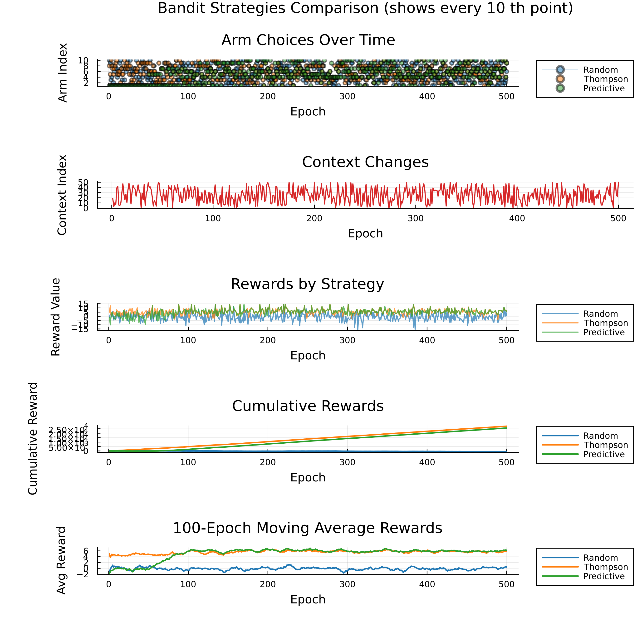
Thompson and Predictive strategies both significantly outperform Random. Both intelligent strategies quickly adapt to changing contexts. The Predictive strategy shows a slight edge over Thompson sampling in final performance, demonstrating the effectiveness of Bayesian approaches in sequential decision-making under uncertainty.
function plot_moving_averages(history, n_epochs, ma_window=20)
    # Calculate moving average rewards
    ma_rewards_random = [mean(history[:rewards][:random][max(1, i - ma_window + 1):i]) for i in 1:n_epochs]
    ma_rewards_thompson = [mean(history[:rewards][:thompson][max(1, i - ma_window + 1):i]) for i in 1:n_epochs]
    ma_rewards_predictive = [mean(history[:rewards][:predictive][max(1, i - ma_window + 1):i]) for i in 1:n_epochs]

    # Plot moving average
    plot(1:n_epochs, [ma_rewards_random, ma_rewards_thompson, ma_rewards_predictive],
        label=["Random" "Thompson" "Predictive"],
        title="Moving Average Reward",
        xlabel="Epoch", ylabel="Average Reward",
        lw=2)
end

# Plot moving averages
plot_moving_averages(history, n_epochs)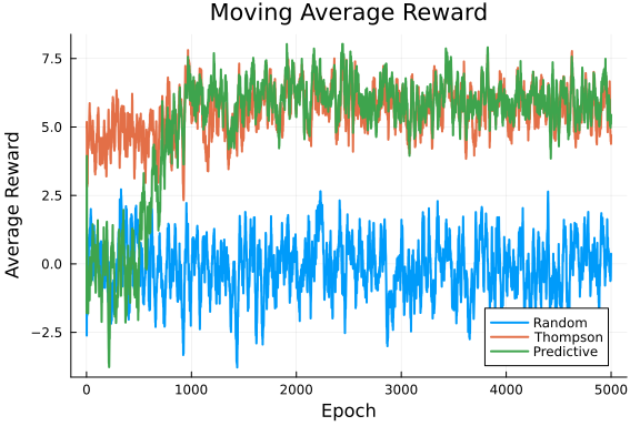
This example was automatically generated from a Jupyter notebook in the RxInferExamples.jl repository.
We welcome and encourage contributions! You can help by:
- Improving this example
- Creating new examples
- Reporting issues or bugs
- Suggesting enhancements
Visit our GitHub repository to get started. Together we can make RxInfer.jl even better! 💪
This example was executed in a clean, isolated environment. Below are the exact package versions used:
For reproducibility:
- Use the same package versions when running locally
- Report any issues with package compatibility
Status `/tmp/jl_kvCR21/Project.toml`
  [31c24e10] Distributions v0.25.126
  [91a5bcdd] Plots v1.41.6
  [92933f4c] ProgressMeter v1.11.0
  [86711068] RxInfer v5.3.4
  [860ef19b] StableRNGs v1.0.4
  [f3b207a7] StatsPlots v0.15.8
  [37e2e46d] LinearAlgebra v1.12.0
  [9a3f8284] Random v1.11.0