This example was automatically generated from a Jupyter notebook in the RxInferExamples.jl repository.
We welcome and encourage contributions! You can help by:
- Improving this example
- Creating new examples
- Reporting issues or bugs
- Suggesting enhancements
Visit our GitHub repository to get started. Together we can make RxInfer.jl even better! 💪
Recurrent Switching Linear Dynamical System
This is an experimental example of a Recurrent Switching Linear Dynamical System (RSLDS) model. The notebook requires patches to RxInfer and ReactiveMP, which are condensed in the hidden blocks below.
Hidden block of RxInfer & ReactiveMP patches and extensions - click to expand
using ExponentialFamily, RxInfer, BayesBase, GraphPPL
using ContinuousTransitionMessagePassingRules, PolyaMessagePassingRules
import ExponentialFamily: getnaturalparameters, exponential_family_typetag

# The Gate node: `out` is the member of the group `inputs` that the one-hot `switch` selects
struct Gate end

# Gate's own algorithm: the messages towards `out` and towards each input read the switch's marginal,
# the message towards `switch` reads the messages on every other edge
struct GateMP <: AbstractAlgorithm end

@define_factor_node(
    node = Gate, type = Deterministic,
    interfaces = [:out, :switch, :inputs...],
    algorithm = GateMP,
    dependencies = [
        :out => (m[:inputs...], q[:switch]),
        :switch => (m[:out], m[:inputs...]),
        (:inputs, k) => (m[:out], q[:switch]),
    ],
)

@define_message_update_rule(
    node = Gate, target = :out,
    args = (m[:inputs...]::Any, q[:switch]::Any),
    body = (args) -> MixtureDistribution(collect(args.m[:inputs]), probvec(args.q[:switch])),
)

@define_message_update_rule(
    node = Gate, target = :switch,
    args = (m[:out]::Any, m[:inputs...]::Any),
    body = (args) -> begin
        m_out = args.m[:out]
        logscales = map(input -> compute_logscale(prod(GenericProd(), m_out, input), m_out, input), args.m[:inputs])
        p = softmax(collect(logscales))
        return Multinomial(1, p)
    end,
)

@define_message_update_rule(
    node = Gate, target = (:inputs, k),
    args = (m[:out]::Any, q[:switch]::Any),
    body = (args) -> begin
        z = probvec(args.q[:switch])[k]
        ef_out = convert(ExponentialFamilyDistribution, args.m[:out])
        η      = getnaturalparameters(ef_out)
        ef_opt = ExponentialFamilyDistribution(exponential_family_typetag(ef_out), η * z)
        return convert(Distribution, ef_opt)
    end,
)

# The joint over the switch and the inputs, for the free energy: their incoming messages, independent
@define_marginal_update_rule(
    node = Gate, target = (:switch, :inputs),
    args = (m[:out]::Any, m[:switch]::Any, m[:inputs...]::Any),
    body = (args) -> FactorizedCluster((:switch,) => args.m[:switch], (:inputs,) => FactorizedJoint(args.m[:inputs])),
)

function BayesBase.prod(::BayesBase.UnspecifiedProd, left::GaussianDistributionsFamily, right::MixtureDistribution)
    comps = BayesBase.components(right)
    weights = BayesBase.weights(right)
    new_comps = []
    for comp in comps
        new_comp = prod(GenericProd(),left, comp)
        push!(new_comps, new_comp)
    end

    return MixtureDistribution(new_comps, weights)
end

BayesBase.prod(::BayesBase.UnspecifiedProd, left::MixtureDistribution, right::GaussianDistributionsFamily) = prod(GenericProd(),right, left)
BayesBase.paramfloattype(::MixtureDistribution) = Float64


import ExponentialFamily.LogExpFunctions: logsumexp
function BayesBase.prod(::GenericProd, left::Categorical, right::Multinomial)
    @assert right.n == 1
    right_cat = Categorical(right.p)

    p = prod(GenericProd(), left, right_cat).p
    return Multinomial(1, p)

end


BayesBase.prod(::GenericProd, left::Multinomial, right::Categorical) = prod(GenericProd(), right, left)
function BayesBase.prod(::GenericProd, left::Multinomial, right::Multinomial)
    @assert left.n == right.n

    p = left.p .* right.p
    p = p ./ sum(p)
    return Multinomial(left.n, p)
end

BayesBase.prod(::BayesBase.UnspecifiedProd, left::Multinomial, right::Multinomial) = prod(GenericProd(), left, right)


function BayesBase.compute_logscale(dist1::Multinomial, dist2::Multinomial, dist3::Multinomial)
    logp1 = log.(dist1.p) - log(dist1.p[end])
    logp2 = log.(dist2.p) - log(dist2.p[end])
    logp3 = log.(dist3.p) - log(dist3.p[end])
    return logsumexp(logp1) - logsumexp(logp2) - logsumexp(logp3)
end

BayesBase.compute_logscale(d1::ExponentialFamily.WishartFast, d2::ExponentialFamily.WishartFast, d3::ExponentialFamily.WishartFast) = begin
    return logpartition(convert(ExponentialFamilyDistribution, d1)) - logpartition(convert(ExponentialFamilyDistribution, d2)) - logpartition(convert(ExponentialFamilyDistribution, d3))
end


ExponentialFamily.probvec(d::Multinomial) = d.p

# ContinuousTransition with a mixture `q(a)`, the output of a Gate: the mixture is moment-matched to a normal
# and the packaged rule is called with it
mixture_to_normal(d) = convert(promote_variate_type(typeof(mean(d)), NormalMeanPrecision), mean(d), precision(d))

@define_message_update_rule(
    node = ContinuousTransition, target = :W, algorithm = CTVMP,
    args = (q[:y, :x]::MultivariateNormalDistributionsFamily, q[:a]::MixtureDistribution),
    body = (algo, ctx, args) -> getresult(call_message_update_rule(ContinuousTransition, :W;
        q = (a = mixture_to_normal(args.q[:a]),), clusters = ((:y, :x) => args.q[:y, :x],), algorithm = algo, ctx)),
)

@define_message_update_rule(
    node = ContinuousTransition, target = :y, algorithm = CTVMP,
    args = (m[:x]::MultivariateNormalDistributionsFamily, q[:a]::MixtureDistribution, q[:W]::Any),
    body = (algo, ctx, args) -> getresult(call_message_update_rule(ContinuousTransition, :y;
        m = (x = args.m[:x],), q = (a = mixture_to_normal(args.q[:a]), W = args.q[:W]), algorithm = algo, ctx)),
)

@define_message_update_rule(
    node = ContinuousTransition, target = :a, algorithm = CTVMP,
    args = (q[:y, :x]::MultivariateNormalDistributionsFamily, q[:a]::MixtureDistribution, q[:W]::Any),
    body = (algo, ctx, args) -> getresult(call_message_update_rule(ContinuousTransition, :a;
        q = (a = mixture_to_normal(args.q[:a]), W = args.q[:W]), clusters = ((:y, :x) => args.q[:y, :x],), algorithm = algo, ctx)),
)

@define_message_update_rule(
    node = ContinuousTransition, target = :x, algorithm = CTVMP,
    args = (m[:y]::MultivariateNormalDistributionsFamily, q[:a]::MixtureDistribution, q[:W]::Any),
    body = (algo, ctx, args) -> getresult(call_message_update_rule(ContinuousTransition, :x;
        m = (y = args.m[:y],), q = (a = mixture_to_normal(args.q[:a]), W = args.q[:W]), algorithm = algo, ctx)),
)

# DiscreteTransition with the `Multinomial(1, p)` messages of MultinomialPolya and the Gate:
# each is the categorical `Categorical(p)`, and the packaged rule is called with it
multinomial_to_categorical(d::Multinomial) = (@assert d.n == 1; Categorical(probvec(d)))

@define_message_update_rule(
    node = DiscreteTransition, target = :out,
    args = (m[:in]::Multinomial, q[:a]::DirichletCollection),
    body = (ctx, args) -> getresult(call_message_update_rule(DiscreteTransition, :out;
        m = (in = multinomial_to_categorical(args.m[:in]),), q = (a = args.q[:a],), ctx)),
)

@define_message_update_rule(
    node = DiscreteTransition, target = :in,
    args = (m[:out]::Multinomial, q[:a]::DirichletCollection),
    body = (ctx, args) -> getresult(call_message_update_rule(DiscreteTransition, :in;
        m = (out = multinomial_to_categorical(args.m[:out]),), q = (a = args.q[:a],), ctx)),
)

@define_marginal_update_rule(
    node = DiscreteTransition, target = (:out, :in),
    args = (m[:out]::Multinomial, m[:in]::Multinomial, q[:a]::DirichletCollection),
    body = (ctx, args) -> getresult(call_marginal_update_rule(DiscreteTransition, (:out, :in);
        m = (out = multinomial_to_categorical(args.m[:out]), in = multinomial_to_categorical(args.m[:in])), q = (a = args.q[:a],), ctx)),
)


Base.length(d::MixtureDistribution) = length(d.components)
Base.ndims(d::MixtureDistribution) = first(size(first(d.components)))

BayesBase.entropy(d::MixtureDistribution) = mapreduce((c,w) -> w * BayesBase.entropy(c), +, d.components, d.weights)

BayesBase.mean(f::F, itr::MixtureDistribution) where {F} = mapreduce((c,w) -> w * mean(f, c), +, itr.components, itr.weights)

function create_P_matrix(n_switches)
    P = zeros(n_switches, n_switches)
    for i in 1:n_switches
        P[i,:] = 0.5 * ones(n_switches)
        P[i,i] = 1.0
    end
    return P
end

function BayesBase.mean(mixture::MixtureDistribution)
    component_means = mean.(BayesBase.components(mixture))
    component_weights = BayesBase.weights(mixture)
    return mapreduce((m,w) -> w*m, +, component_means, component_weights)
end

function BayesBase.cov(mixture::MixtureDistribution)
    component_cov = cov.(BayesBase.components(mixture))
    component_means = mean.(BayesBase.components(mixture))
    component_weights = BayesBase.weights(mixture)
    mixture_mean = mean(mixture)
    return mapreduce((v,m,w) -> w*(v + m*m'), +, component_cov, component_means, component_weights) - mixture_mean*mixture_mean'
end

BayesBase.precision(mixture::MixtureDistribution) = inv(cov(mixture))

function BayesBase.var(mixture::MixtureDistribution)
    component_vars = var.(BayesBase.components(mixture))
    component_means = mean.(BayesBase.components(mixture))
    component_weights = BayesBase.weights(mixture)
    mixture_mean = mean(mixture)
    return mapreduce((v,m,w) -> w*(v + m.^2), +, component_vars, component_means, component_weights) - mixture_mean.^2
end
Hidden block of RSLDS Model Specification - click to expand
import ExponentialFamily: softmax

"""
    RSLDSHyperparameters{T}

Structure containing hyperparameters for the Recurrent Switching Linear Dynamical System (RSLDS) model.

# Fields
- `a_w::T = 2.0`: Shape parameter for the Gamma prior on precision parameter w (when n_switches=1)
- `b_w::T = 2.0`: Rate parameter for the Gamma prior on precision parameter w (when n_switches=1)
- `Ψ_w::Matrix{T}`: Scale matrix for the Wishart prior on precision matrix w (when n_switches>1)
- `Ψ_R::Union{Matrix{T}, T}`: Scale matrix/parameter for the Wishart/Gamma prior on observation precision
- `ν_R::T`: Degrees of freedom for the Wishart prior on observation precision
- `α::Matrix{T}`: Parameter matrix for the Dirichlet prior on transition probabilities
- `C::Matrix{T}`: Observation matrix mapping latent states to observations
"""
Base.@kwdef struct RSLDSHyperparameters{T}
   a_w::T = 2.0
   b_w::T = 2.0
   Ψ_w::Matrix{T}
   Ψ_R::Union{Matrix{T}, T}
   ν_R::T
   α::Matrix{T}
   C::Matrix{T}
end

"""
    get_hyperparameters(hyperparameters::RSLDSHyperparameters)

Extract all hyperparameters from the RSLDSHyperparameters structure.

# Arguments
- `hyperparameters::RSLDSHyperparameters`: Structure containing the hyperparameters

# Returns
A tuple containing all hyperparameters in the order: a_w, b_w, Ψ_w, Ψ_R, ν_R, α, C
"""
function get_hyperparameters(hyperparameters::RSLDSHyperparameters)
    return hyperparameters.a_w, hyperparameters.b_w, hyperparameters.Ψ_w, hyperparameters.Ψ_R, hyperparameters.ν_R, hyperparameters.α, hyperparameters.C
end

"""
    default_hyperparameters(n_switches, obs_dim, dim_latent)

Create a default set of hyperparameters for the RSLDS model.

# Arguments
- `n_switches`: Number of switching states in the model
- `obs_dim`: Dimension of the observation space
- `dim_latent`: Dimension of the latent state space

# Returns
An RSLDSHyperparameters structure with default values
"""
function default_hyperparameters(n_switches, obs_dim, dim_latent)
    return RSLDSHyperparameters(
        a_w = 2.0,
        b_w = 2.0,
        Ψ_w = diageye(n_switches),
        Ψ_R = diageye(obs_dim),
        ν_R = obs_dim + 2.0,
        α = ones(n_switches+1, n_switches+1),
        C = diageye(obs_dim,dim_latent)
    )
end


@model function rslds_model_learning(obs,n_obs,n_switches, dim_latent, η, Ψ, hyperparameters, learn_observation_covariance)
    local H,A,Λ,u
    transformation  = (x) -> reshape(x, (dim_latent, dim_latent))
    transformation2 = (x) -> reshape(x, (n_switches, dim_latent))
    ##Hyperparameters
    a_w, b_w, Ψ_w, Ψ_R,ν_R, α, C = get_hyperparameters(hyperparameters)
    ## Priors on the parameters
    if n_switches == 1
        w ~ GammaShapeRate(a_w, b_w)
    else
        w ~ Wishart(n_switches+2,Ψ_w)
    end

    if learn_observation_covariance
        if n_obs == 1
            R ~ GammaShapeRate(ν_R, Ψ_R)
        else
            R ~ Wishart(ν_R, Ψ_R)
        end
    else
        R = Ψ_R
    end

    for k in 1:n_switches+1
        H[k] ~ MvNormalMeanCovariance(zeros(dim_latent^2), diageye(dim_latent^2))
        Λ[k] ~ Wishart(dim_latent+2, diageye(dim_latent))
    end
    P ~ DirichletCollection(α)
    ϕ ~ MvNormalMeanCovariance(zeros(dim_latent*n_switches), diageye(dim_latent*n_switches))
    ## States Initialisation
    x[1] ~ MvNormalMeanCovariance(zeros(dim_latent), diageye(dim_latent))
    for t in eachindex(obs)
        ## Recurrent Layer
        if n_switches == 1
            u[t] ~ softdot(ϕ, x[t], w)
        else
            u[t] ~ ContinuousTransition(x[t], ϕ, w) where {algorithm = CTVMP(transformation2)}
        end
        s[t] ~ MultinomialPolya(1, u[t]) where {initial_messages = (ψ = convert(promote_variate_type(typeof(η), NormalWeightedMeanPrecision), η, Ψ),)}
        s[t+1] ~ DiscreteTransition(s[t], P)
        ##Transition Layer
        A[t] := Gate(switch=s[t+1], inputs=H)
        B[t] := Gate(switch=s[t+1], inputs=Λ)
        x[t+1] ~ ContinuousTransition(x[t], A[t], B[t]) where {algorithm = CTVMP(transformation)}
        ## Observation Layer
        obs[t] ~ MvNormalMeanPrecision(C*x[t+1], R)
    end
end

@constraints  function rslds_learning_constraints(learn_observation_covariance)
    if learn_observation_covariance
        q(x,s,u,ϕ,w,P,H,A,Λ,B,R) = q(x,u)q(A)q(s)q(ϕ)q(w)q(P)q(H)q(Λ)q(B)q(R)
    else
        q(x,s,u,ϕ,w,P,H,A,Λ,B) = q(x,u)q(A)q(s)q(ϕ)q(w)q(P)q(H)q(Λ)q(B)
    end
end

@initialization function rslds_learning_initmarginals(n_switches, dim_latent, obs_dim, learn_observation_covariance; rng = StableRNG(42))
    q(x) = vague(MvNormalWeightedMeanPrecision, dim_latent)
    q(s) = Multinomial(1,softmax(randn(rng, n_switches+1)))
    q(ϕ) = vague(MvNormalWeightedMeanPrecision, dim_latent*(n_switches))
    if n_switches == 1
        q(w) = vague(GammaShapeRate)
    else
        q(w) = vague(Wishart, n_switches)
    end
    q(A) = vague(MvNormalWeightedMeanPrecision, dim_latent^2)
    q(P) = DirichletCollection(ones(n_switches+1,n_switches+1))
    q(Λ) = vague(Wishart, dim_latent)
    q(H) = vague(MvNormalWeightedMeanPrecision, dim_latent^2)
    q(B) = vague(Wishart, dim_latent)
    if learn_observation_covariance
        if obs_dim == 1
            q(R) = vague(GammaShapeRate)
        else
            q(R) = Wishart(obs_dim+2, diageye(obs_dim))
        end
    end
end;


"""
    fit_rslds(data, n_switches, dim_latent, n_obs; kwargs...)

Fit a Recurrent Switching Linear Dynamical System (RSLDS) model to the provided data.

# Arguments
- `data`: Time series observation data
- `n_switches`: Number of switching states in the model. Note: The user provides the total number of states,
  but internally we use (n_switches-1) because the MultinomialPolya distribution adds an extra dimension
  to represent the recurrent influence on state transitions.
- `dim_latent`: Dimension of the latent state space
- `n_obs`: Dimension of the observation space

# Keyword Arguments
- `iterations::Int = 60`: Number of inference iterations
- `η = nothing`: Mean parameter of the initial message on MultinomialPolya's `ψ`
- `Ψ = nothing`: Precision parameter of the initial message on MultinomialPolya's `ψ`
- `hyperparameters = nothing`: Custom hyperparameters for the model
- `progress::Bool = false`: Whether to show progress during inference
- `learn_observation_covariance::Bool = false`: Whether to learn the observation covariance

# Returns
The result of the inference procedure
"""
function fit_rslds(data, n_switches, dim_latent, n_obs; iterations = 60, η = nothing, Ψ = nothing, hyperparameters = nothing, progress = false, learn_observation_covariance = false)
    @assert n_switches > 1 "n_switches must be greater than 1"
    # We subtract 1 from n_switches because the MultinomialPolya distribution
    # internally adds an extra dimension to represent the recurrent influence
    # on state transitions. This convention allows the model to maintain the
    # correct dimensionality while incorporating the recurrent dynamics.
    n_switches = n_switches - 1

    if hyperparameters === nothing
        hyperparameters = default_hyperparameters(n_switches, length(data[1]), dim_latent)
    end

    if η === nothing
        if n_switches == 1
            η = 0.0
        else
            η = zeros(n_switches)
        end
    end
    if Ψ === nothing
        if n_switches == 1
            Ψ = 0.0001
        else
            Ψ = 0.0001*diageye(n_switches)
        end
    end
    model = rslds_model_learning(n_obs = n_obs, n_switches = n_switches, dim_latent = dim_latent, η = η, Ψ = Ψ, hyperparameters = hyperparameters, learn_observation_covariance = learn_observation_covariance)
    constraints = rslds_learning_constraints(learn_observation_covariance)
    initmarginals = rslds_learning_initmarginals(n_switches, dim_latent, n_obs, learn_observation_covariance)

    return infer(model = model, data = (obs=data, ), constraints = constraints, initialization = initmarginals, iterations = iterations,
    showprogress = progress,
    returnvars = KeepEach(),
    free_energy = true,
    options = (limit_stack_depth = 100,)
    )
end

#

function states_to_categorical(states)
    return [argmax(states[t].p) for t in 1:length(states)]
end
Hidden block of Generating Synthetic Data - click to expand
using StableRNGs

function generate_switching_data(T, A1, A2, c, Q, R, x_0;rng = StableRNG(42))
    # Initialize arrays to store states and observations
    x = zeros(2, T)  # State matrix: 2 dimensions × T timesteps
    y = zeros(2, T)  # Observation matrix: 2 dimensions × T timesteps

    # Set initial state
    x[:,1] = x_0

    # Generate state transitions and observations
    for t in 2:T
        # Switch dynamics multiple times through the sequence
        if t < T/3 || (t >= T/2 && t < 3T/4)
            x[:,t] = A2 * x[:,t-1] + rand(rng,MvNormal(zeros(2), Q))  # First regime
        else
            x[:,t] = A1 * x[:,t-1] + rand(rng,MvNormal(zeros(2), Q))  # Second regime
        end

        # Generate observation from current state
        y[:,t] = c * x[:,t] + rand(rng,MvNormal(zeros(2), R))
    end

    return x, y
end


# System parameters
T = 500  # Time horizon
θ = π / 15  # Rotation angle

# Define system matrices
A1 = [cos(θ) -sin(θ); sin(θ) cos(θ)]    # Rotation matrix
A2 = [0.4 -0.01; 0.01 0.2]
c = [0.6 -0.02; -0.02 0.3]                   # Observation/distortion matrix

# Noise parameters
Q = [1.0 0.0; 0.0 1.0]                   # State noise covariance
R =  [1.0 0.0; 0.0 1.0]            # Observation noise variance
x_0 = [0.0, 0.0]                         # Initial state vector

# Generate synthetic data
x, y = generate_switching_data(T, A1, A2, c, Q, R, x_0)
y = [y[:,i] for i in 1:T]
x = [x[:,i] for i in 1:T]
hyperparameters = RSLDSHyperparameters(
    a_w = 0.01,
    b_w = 0.01,
    Ψ_w = 10.0*diageye(2), # n-1
    Ψ_R = inv(R),
    ν_R = 4.0,
    α = ones(2,2), # n
    C = c
)
Main.var"##WeaveSandBox#142".RSLDSHyperparameters{Float64}(0.01, 0.01, [10.
0 0.0; 0.0 10.0], [1.0 0.0; 0.0 1.0], 4.0, [1.0 1.0; 1.0 1.0], [0.6 -0.02;
-0.02 0.3])
rslds_result = fit_rslds(y, 2, 2, 2; iterations = 150, hyperparameters = hyperparameters, progress = true)
Inference results:
  Posteriors       | available for (ϕ, w, P, A, s, H, Λ, B, u, x)
  Free Energy:     | [33649.8, 6095.3, 4237.16, 3999.39, 3962.24, 3943.03,
3923.13, 3906.84, 3893.2, 3880.78  …  1950.64, 1950.61, 1950.58, 1950.55, 1
950.52, 1950.5, 1950.47, 1950.44, 1950.42, 1950.39]
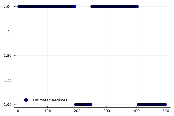
using Plots
switching_state_posterior = rslds_result.posteriors[:s][end];
states = states_to_categorical(switching_state_posterior);
scatter(states, label="Estimated Regimes", color="blue", linewidth=2)
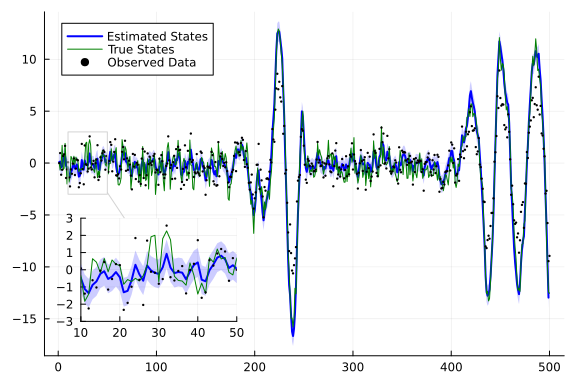
continuous_state_posterior = rslds_result.posteriors[:x][end];
index = 1
from = 1
to = 500

m_continuous = getindex.(mean.(continuous_state_posterior), index);
var_continuous = getindex.(var.(continuous_state_posterior), index);
plot(m_continuous[from+1:to], ribbon=sqrt.(var_continuous[from+1:to]), label="Estimated States", color="blue",fillalpha=0.2, linewidth=2)
plot!(getindex.(x,index)[from:to], label="True States", color="green", linewidth=1)
scatter!(getindex.(y,index)[from:to], label="Observed Data", color="black", ms=1.3)
lens!([10,50],[-3, 3],inset = (1, bbox(0.07, 0.6, 0.3, 0.3)), )
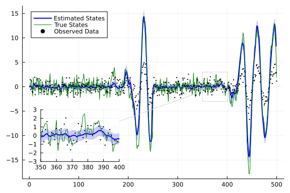
index = 2
m_continuous = getindex.(mean.(continuous_state_posterior), index);
var_continuous = getindex.(var.(continuous_state_posterior), index);
plot(m_continuous[from+1:to], ribbon=sqrt.(var_continuous[from+1:to]), label="Estimated States", color="blue",fillalpha=0.2, linewidth=2)
plot!(getindex.(x,index)[from:to], label="True States", color="green", linewidth=1)
scatter!(getindex.(y,index)[from:to], label="Observed Data", color="black", ms=1.3)
lens!([350,400],[-3, 3],inset = (1, bbox(0.07, 0.6, 0.3, 0.3)), )
println("Estimated continuous transition matrices:")
println("----------------------------------------")
for i in 1:length(rslds_result.posteriors[:H][end])
    println("Matrix $i:")
    println(reshape(mean(rslds_result.posteriors[:H][end][i]), 2, 2))
    println()
end
Estimated continuous transition matrices:
----------------------------------------
Matrix 1:
[0.9803317173470955 -0.20982789659577544; 0.19037190350089697 0.97935728060
80625]

Matrix 2:
[0.5061888709542391 -0.3235960880634839; 0.10734100727773228 0.534224400370
062]println("Estimated discrete transition matrix for HMM layer:")
println("----------------------------------------")
println(mean(rslds_result.posteriors[:P][end]))
Estimated discrete transition matrix for HMM layer:
----------------------------------------
[0.9866129184532206 0.008637334648914212; 0.013387081546779412 0.9913626653
510859]This example was automatically generated from a Jupyter notebook in the RxInferExamples.jl repository.
We welcome and encourage contributions! You can help by:
- Improving this example
- Creating new examples
- Reporting issues or bugs
- Suggesting enhancements
Visit our GitHub repository to get started. Together we can make RxInfer.jl even better! 💪
This example was executed in a clean, isolated environment. Below are the exact package versions used:
For reproducibility:
- Use the same package versions when running locally
- Report any issues with package compatibility
Status `/tmp/jl_LCtdtQ/Project.toml`
  [b4ee3484] BayesBase v1.5.12
  [be169b08] ContinuousTransitionMessagePassingRules v1.0.0
  [62312e5e] ExponentialFamily v2.9.0
  [b3f8163a] GraphPPL v4.9.0
  [91a5bcdd] Plots v1.41.7
  [2d94fc58] PolyaMessagePassingRules v1.0.0
  [86711068] RxInfer v6.1.1
  [860ef19b] StableRNGs v1.1.0