This example was automatically generated from a Jupyter notebook in the RxInferExamples.jl repository.
We welcome and encourage contributions! You can help by:
- Improving this example
- Creating new examples
- Reporting issues or bugs
- Suggesting enhancements
Visit our GitHub repository to get started. Together we can make RxInfer.jl even better! 💪
Bayesian Multinomial Regression
This notebook is an introductory tutorial to Bayesian multinomial regression with RxInfer.
using RxInfer, Plots, StableRNGs, Distributions, ExponentialFamily, StatsPlots
import ExponentialFamily: softmax
Model Description
The key innovation in Linderman et al. (2015) is extending the Pólya-gamma augmentation scheme to the multinomial case. This allows us to transform the non-conjugate multinomial likelihood into a conditionally conjugate form by introducing auxiliary Pólya-gamma random variables.
The multinomial regression model with Pólya-gamma augmentation can be written as: $p(y | \psi, N) = \text{Multinomial}(y |N, \psi)$
where:
\[y\]
is a $K$-dimensional vector of count data with $N$ total counts\[\psi\]
is a $K-1$ -dimensional Gaussian random variable
Implementation
In this notebook, we will implement the Pólya-gamma augmented Bayesian multinomial regression model with RxInfer by performing inference using message passing to estimate the posterior distribution of the regression coefficients
function generate_multinomial_data(rng=StableRNG(123);N = 20, k=9, nsamples = 1000)
    Ψ = randn(rng, k)
    p = softmax(Ψ)
    X = rand(rng, Multinomial(N, p), nsamples)
    X= [X[:,i] for i in 1:size(X,2)];
    return X, Ψ,p
end
generate_multinomial_data (generic function with 2 methods)nsamples = 5000
N = 30
k = 40
X, Ψ, p = generate_multinomial_data(N=N,k=k,nsamples=nsamples);The MultinomialPolya factor node is used to model the likelihood of the multinomial distribution.
Due to non-conjugacy of the likelihood and the prior distribution, we need to use a more complex inference algorithm. RxInfer provides an Expectation Propagation (EP) [2] algorithm to infer the posterior distribution. Due to EP's approximation, we need to specify an inbound message for the regression coefficients while using the MultinomialPolya factor node. This feature is implemented in the dependencies keyword argument during the creation of the MultinomialPolya factor node. ReactiveMP.jl provides a RequireMessageFunctionalDependencies type that is used to specify the inbound message for the regression coefficients ψ. Refer to the ReactiveMP.jl documentation for more information.
@model function multinomial_model(obs, N, ξ_ψ, W_ψ)
    ψ ~ MvNormalWeightedMeanPrecision(ξ_ψ, W_ψ)
    obs .~ MultinomialPolya(N, ψ) where {dependencies = RequireMessageFunctionalDependencies(ψ = MvNormalWeightedMeanPrecision(ξ_ψ, W_ψ))}
end
result = infer(
model = multinomial_model(ξ_ψ=zeros(k-1), W_ψ=rand(Wishart(3, diageye(k-1))), N=N),
data = (obs=X, ),
iterations = 50,
free_energy = true,
showprogress = true,
options = (
limit_stack_depth = 100,
)
)Inference results:
Posteriors | available for (ψ)
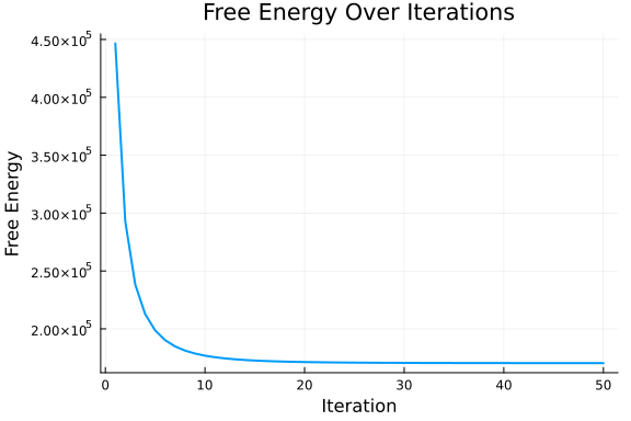
Free Energy: | Real[4.46367e5, 2.92489e5, 2.37944e5, 2.12213e5, 1.981
22e5, 1.89646e5, 1.84203e5, 1.80534e5, 1.77966e5, 1.76114e5 … 1.69521e5,
1.69513e5, 1.69507e5, 169501.0, 1.69496e5, 1.69491e5, 169487.0, 1.69483e5,
1.6948e5, 169477.0]plot(result.free_energy[1:end],
title="Free Energy Over Iterations",
xlabel="Iteration",
ylabel="Free Energy",
linewidth=2,
legend=false,
grid=true,
)
predictive = @call_rule MultinomialPolya(:x, Marginalisation) (q_N = PointMass(N), q_ψ = result.posteriors[:ψ][end], meta = MultinomialPolyaMeta(21))
println("Estimated data generation probabilities: $(predictive.p)")
println("True data generation probabilities: $(p)")
Estimated data generation probabilities: [0.012128530184393771, 0.027656076
01446005, 0.004660891444039877, 0.012701237710875455, 0.013549812317938958,
0.03737878325421617, 0.007645347861696176, 0.007065856341489352, 0.0057004
85469805119, 0.004209560941872535, 0.005429993146293316, 0.0036292423953019
804, 0.004096647759833256, 0.03647926577305119, 0.10854880835010822, 0.0725
4127770162921, 0.026434420343417878, 0.024052548272387567, 0.01034033908660
0318, 0.008755289933567624, 0.04015814397083516, 0.0048429009095223765, 0.0
08225370359180724, 0.026499659850507295, 0.006638855420325549, 0.0082071128
03766426, 0.008963212226224712, 0.007190673235254259, 0.01713461259123492,
0.00732486491378469, 0.008876369774876446, 0.0035821590712402204, 0.0112094
15492110856, 0.010548425909739511, 0.0949119666608159, 0.04410888974581073,
0.13264612770612946, 0.027591466728893753, 0.030292633787168927, 0.0680427
2453959984]
True data generation probabilities: [0.012475572764691347, 0.02759115956301
153, 0.004030932560100506, 0.013008651265311708, 0.012888510278451618, 0.03
7656116813111006, 0.007242363105598982, 0.006930069564505769, 0.00538389836
228327, 0.0036198124274772225, 0.005212387391120808, 0.003185556887255863,
0.003820168769118259, 0.036849638787622915, 0.109428569898501, 0.0726075387
5224316, 0.026079268674281158, 0.024477855252934583, 0.010207778995219957,
0.008532295265944583, 0.040242532118754906, 0.005181587450423221, 0.0082073
91370854009, 0.02741148713822125, 0.006623087410725917, 0.00836770271463416
2, 0.009668643362989908, 0.007171783607096945, 0.016985615150215773, 0.0070
80691453323701, 0.008297044496975403, 0.0037359000700039487, 0.011142755810
390478, 0.010256554277897088, 0.09528238587772694, 0.04369806970660494, 0.1
3308101804159636, 0.02665693577960761, 0.030479170124456504, 0.069201498658
71575]mse = mean((predictive.p - p).^2);
println("MSE between estimated and true data generation probabilities: $mse")MSE between estimated and true data generation probabilities: 2.03098748471
75222e-7@model function multinomial_regression(obs, N, X, ϕ, ξβ, Wβ)
β ~ MvNormalWeightedMeanPrecision(ξβ, Wβ)
for i in eachindex(obs)
Ψ[i] := ϕ(X[i])*β
obs[i] ~ MultinomialPolya(N, Ψ[i]) where {dependencies = RequireMessageFunctionalDependencies(ψ = MvNormalWeightedMeanPrecision(zeros(length(obs[i])-1), diageye(length(obs[i])-1)))}
end
endfunction generate_regression_data(rng=StableRNG(123);ϕ = identity,N = 3, k=5, nsamples = 1000)
β = randn(rng, k)
X = randn(rng, nsamples, k, k)
X = [X[i,:,:] for i in 1:size(X,1)];
Ψ = ϕ.(X)
p = map(x -> logistic_stick_breaking(x*β), Ψ)
return map(x -> rand(rng, Multinomial(N, x)), p), X, β, p
endgenerate_regression_data (generic function with 2 methods)ϕ = x -> sin(x)
obs_regression, X_regression, β_regression, p_regression = generate_regression_data(;nsamples = 5000, ϕ = ϕ);reg_results = infer(
model = multinomial_regression(N = 3, ϕ = ϕ, ξβ = zeros(5), Wβ = rand(Wishart(5, diageye(5)))),
data = (obs=obs_regression,X = X_regression ),
iterations = 20,
free_energy = true,
showprogress = true,
returnvars = KeepLast(),
options = (
limit_stack_depth = 100,
)
)Inference results:
Posteriors | available for (Ψ, β)
Free Energy: | Real[11953.9, 11590.0, 11508.6, 11487.9, 11482.4, 1148
0.9, 11480.4, 11480.3, 11480.3, 11480.3, 11480.3, 11480.3, 11480.3, 11480.3
, 11480.3, 11480.3, 11480.3, 11480.3, 11480.3, 11480.3]println("estimated β: with mean and covariance: $(mean_cov(reg_results.posteriors[:β]))")
println("true β: $(β_regression)")estimated β: with mean and covariance: ([-0.11310143983943352, 0.6606354999
509866, -1.250329655401701, -0.08350492996067109, -0.07948711146379472], [0
.0001477926670120436 -2.1383295631058373e-6 3.3961821081765535e-6 -1.692234
7608420979e-6 3.2125506409672206e-6; -2.1383295631058373e-6 0.0001513890200
8181383 -1.9104267228869203e-5 -1.62093322389142e-7 1.2839328043376111e-6;
3.3961821081765535e-6 -1.9104267228869203e-5 0.00017930003375264894 4.23765
3654657978e-6 4.538452315758226e-7; -1.6922347608420979e-6 -1.6209332238914
2e-7 4.237653654657978e-6 0.00013997308596009074 3.1605098980547617e-6; 3.2
125506409672206e-6 1.2839328043376111e-6 4.538452315758226e-7 3.16050989805
47617e-6 0.00013932868262693873])
true β: [-0.12683768965424458, 0.6668851724871252, -1.2566124895590247, -0.
08499562516549662, -0.094274004848194]plot(reg_results.free_energy,
title="Free Energy Over Iterations",
xlabel="Iteration",
ylabel="Free Energy",
linewidth=2,
legend=false,
grid=true,)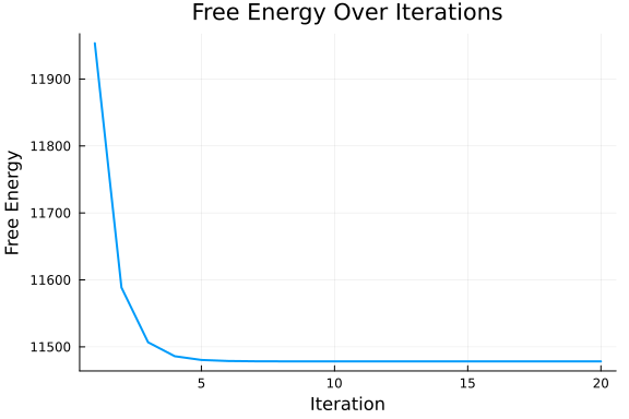
mse_β =  mean((mean(reg_results.posteriors[:β]) - β_regression).^2)
println("MSE of β estimate: $mse_β")
MSE of β estimate: 9.761827179751463e-5We can visualize how the logistic stick-breaking transformation of the simplex coordinates of the regression coefficients affects the prior distribution of the regression coefficients and vice versa since the logistic stick-breaking transformation is invertible.
# Previous helper functions remain the same
σ(x) = 1 / (1 + exp(-x))
σ_inv(x) = log(x / (1 - x))

function jacobian_det(π)
    K = length(π)
    det = 1.0
    for k in 1:(K-1)
        num = 1 - sum(π[1:(k-1)])
        den = π[k] * (1 - sum(π[1:k]))
        det *= num / den
    end
    return det
end

function ψ_to_π(ψ::Vector{Float64})
    K = length(ψ) + 1
    π = zeros(K)
    for k in 1:(K-1)
        π[k] = σ(ψ[k]) * (1 - sum(π[1:(k-1)]))
    end
    π[K] = 1 - sum(π[1:(K-1)])
    return π
end

function π_to_ψ(π)
    K = length(π)
    ψ = zeros(K-1)
    ψ[1] = σ_inv(π[1])
    for k in 2:(K-1)
        ψ[k] = σ_inv(π[k] / (1 - sum(π[1:(k-1)])))
    end
    return ψ
end

# Function to compute density in simplex coordinates
function compute_simplex_density(x::Float64, y::Float64, Σ::Matrix{Float64})
    # Check if point is inside triangle
    if y < 0 || y > 1 || x < 0 || x > 1 || (x + y) > 1
        return 0.0
    end

    # Convert from simplex coordinates to π
    π1 = x
    π2 = y
    π3 = 1 - x - y

    try
        ψ = π_to_ψ([π1, π2, π3])
        # Compute Gaussian density
        dist = MvNormal(zeros(2), Σ)
        return pdf(dist, ψ) * abs(jacobian_det([π1, π2, π3]))
    catch
        return 0.0
    end

end

function plot_transformed_densities()
    # Create three different covariance matrices
    ###For higher variances values needs scaling for proper visualization.
    σ² = 1.0
    Σ_corr = [σ² 0.9σ²; 0.9σ² σ²]
    Σ_anticorr = [σ² -0.9σ²; -0.9σ² σ²]
    Σ_uncorr = [σ² 0.0; 0.0 σ²]

    # Plot Gaussian densities
    ψ1, ψ2 = range(-4sqrt(σ²), 4sqrt(σ²), length=500), range(-4sqrt(σ²), 4sqrt(σ²), length=100)

    p1 = contour(ψ1, ψ2, (x,y) -> pdf(MvNormal(zeros(2), Σ_corr), [x,y]),
                 title="Correlated Prior", xlabel="ψ₁", ylabel="ψ₂")
    p2 = contour(ψ1, ψ2, (x,y) -> pdf(MvNormal(zeros(2), Σ_anticorr), [x,y]),
                 title="Anti-correlated Prior", xlabel="ψ₁", ylabel="ψ₂")
    p3 = contour(ψ1, ψ2, (x,y) -> pdf(MvNormal(zeros(2), Σ_uncorr), [x,y]),
                 title="Uncorrelated Prior", xlabel="ψ₁", ylabel="ψ₂")

    # Plot simplex densities
    n_points = 500
    x = range(0, 1, length=n_points)
    y = range(0, 1, length=n_points)

    # Plot simplices
    p4 = contour(x, y, (x,y) -> compute_simplex_density(x, y, Σ_corr),
                 title="Correlated Simplex")

    # Add simplex boundaries and median lines
    plot!(p4, [0,1,0,0], [0,0,1,0], color=:black, label="")  # Triangle boundaries

    p5 = contour(x, y, (x,y) -> compute_simplex_density(x, y, Σ_anticorr),
                 title="Anti-correlated Simplex")
    plot!(p5, [0,1,0,0], [0,0,1,0], color=:black, label="")

    p6 = contour(x, y, (x,y) -> compute_simplex_density(x, y, Σ_uncorr),
                 title="Uncorrelated Simplex")
    plot!(p6, [0,1,0,0], [0,0,1,0], color=:black, label="")

    # Combine all plots
    plot(p1, p2, p3, p4, p5, p6, layout=(2,3), size=(900,600))
end

# Generate the plots
plot_transformed_densities()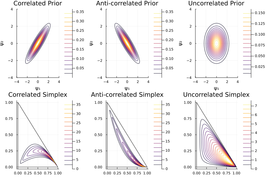
This example was automatically generated from a Jupyter notebook in the RxInferExamples.jl repository.
We welcome and encourage contributions! You can help by:
- Improving this example
- Creating new examples
- Reporting issues or bugs
- Suggesting enhancements
Visit our GitHub repository to get started. Together we can make RxInfer.jl even better! 💪
This example was executed in a clean, isolated environment. Below are the exact package versions used:
For reproducibility:
- Use the same package versions when running locally
- Report any issues with package compatibility
Status `/tmp/jl_kvCR21/Project.toml`
  [31c24e10] Distributions v0.25.126
  [62312e5e] ExponentialFamily v2.4.0
  [91a5bcdd] Plots v1.41.6
  [86711068] RxInfer v5.3.4
  [860ef19b] StableRNGs v1.0.4
  [f3b207a7] StatsPlots v0.15.8