This example was automatically generated from a Jupyter notebook in the RxInferExamples.jl repository.
We welcome and encourage contributions! You can help by:
- Improving this example
- Creating new examples
- Reporting issues or bugs
- Suggesting enhancements
Visit our GitHub repository to get started. Together we can make RxInfer.jl even better! 💪
Integrating Neural Networks with Lux.jl
This advanced tutorial mirrors the Flux.jl example on the same Lorenz state-space problem, but uses Lux.jl — a pure-functional neural network library — together with Optimisers.jl for parameter updates. Everything else (the RxInfer model, the inference-as-training loss, the AD backend) is the same as the Flux version, which makes the two notebooks directly comparable.
using RxInfer, Lux, Optimisers, Random, Plots, LinearAlgebra, StableRNGs, ForwardDiffIn this example, our focus is on Bayesian state estimation in a Nonlinear State-Space Model with unknown dynamics. The main challenge in this scenario is that the dynamics of the system are often unknown or too complex to model analytically. Traditional approaches might struggle with capturing the nonlinear relationships in such systems. Neural networks offer a powerful solution by learning these complex dynamics directly from data, but incorporating them into a Bayesian framework requires careful integration to maintain probabilistic interpretations and uncertainty quantification. This tutorial demonstrates how to overcome these challenges by combining the flexibility of neural networks with the principled uncertainty handling of probabilistic programming. Specifically, we will utilize the time series generated by the Lorenz system as an example.
# Lorenz system equations to be used to generate dataset
Base.@kwdef mutable struct Lorenz
    dt::Float64
    σ::Float64
    ρ::Float64
    β::Float64
    x::Float64
    y::Float64
    z::Float64
end

# Define the Lorenz dynamics
function step!(l::Lorenz)
    dx = l.σ * (l.y - l.x);         l.x += l.dt * dx
    dy = l.x * (l.ρ - l.z) - l.y;   l.y += l.dt * dy
    dz = l.x * l.y - l.β * l.z;     l.z += l.dt * dz
end

function create_dataset(rng, σ, ρ, β_nom; variance = 1f0, n_steps = 100, p_train = 0.8, p_test = 0.2)
    attractor = Lorenz(0.02, σ, ρ, β_nom/3.0, 1, 1, 1)
    signal       = [Float32[1.0, 1.0, 1.0]]
    noisy_signal = [last(signal) + randn(rng, Float32, 3) * variance]
    for i in 1:(n_steps - 1)
        step!(attractor)
        push!(signal, Float32[attractor.x, attractor.y, attractor.z])
        push!(noisy_signal, last(signal) + randn(rng, Float32, 3) * variance)
    end

    return (
        parameters = (σ, ρ, β_nom),
        signal = signal,
        noisy_signal = noisy_signal
    )
end
create_dataset (generic function with 1 method)rng = StableRNG(999) # dummy rng
variance = 2f0
dataset = create_dataset(rng, 11, 23, 6; variance = variance, n_steps = 200);The dataset generated above represents the Lorenz system, a well-known chaotic dynamical system. We've created both clean trajectories following the exact Lorenz equations and noisy observations by adding Gaussian noise with variance 2.0. The dataset contains 200 time steps, providing sufficient data to train our neural network model. The parameters used for this Lorenz system are σ=11, ρ=23, and β=6. This noisy dataset will allow us to test our neural network's ability to filter out noise and recover the underlying dynamics.
# Extract first samples from datasets
sample_clean = dataset.signal
sample_noisy = dataset.noisy_signal

# Pre-allocate arrays for better performance
n_points = length(sample_clean)
gx, gy, gz = zeros(n_points), zeros(n_points), zeros(n_points)
rx, ry, rz = zeros(n_points), zeros(n_points), zeros(n_points)

# Extract coordinates
for i in 1:n_points
    # Noisy observations
    rx[i], ry[i], rz[i] = sample_noisy[i][1], sample_noisy[i][2], sample_noisy[i][3]
    # True state
    gx[i], gy[i], gz[i] = sample_clean[i][1], sample_clean[i][2], sample_clean[i][3]
end

# Create three projection plots
p1 = scatter(rx, ry, label="Noisy observations", alpha=0.7, markersize=2, title = "X-Y Projection")
plot!(p1, gx, gy, label="True state", linewidth=2)

p2 = scatter(rx, rz, label="Noisy observations", alpha=0.7, markersize=2, title = "X-Z Projection")
plot!(p2, gx, gz, label="True state", linewidth=2)

p3 = scatter(ry, rz, label="Noisy observations", alpha=0.7, markersize=2, title = "Y-Z Projection")
plot!(p3, gy, gz, label="True state", linewidth=2)

# Combine plots with improved layout
plot(p1, p2, p3, size=(900, 250), layout=(1,3), margin=5Plots.mm)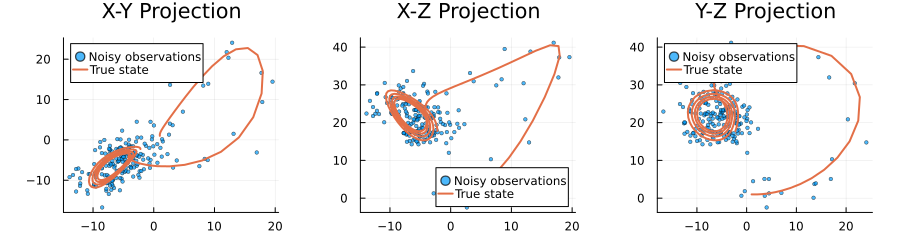
The plots above visualize our noisy Lorenz system dataset from three different perspectives. We can clearly see how the noise (represented by the scattered points) obscures the true underlying dynamics (shown by the solid lines). The Lorenz system's characteristic butterfly-shaped attractor is visible in these projections, though the noisy observations make it challenging to discern the exact trajectory. This visualization highlights the challenge our neural network will face: it must learn to filter out the Gaussian noise (with variance 2.0) and recover the true state of the system at each time step. The X-Y, X-Z, and Y-Z projections each provide a different view of the same 3D dynamical system, helping us understand the full complexity of the dataset.
Bayesian Inference meets Neural Networks
Our objective is to compute the marginal posterior distribution of the latent (hidden) state $x_k$ at each time step $k$, considering the history of measurements up to that time step:
\[p(x_k | y_{1:k}).\]
The above expression represents the probability distribution of the latent state $x_k$ given the measurements $y_{1:k}$ up to time step $k$. The hidden dynamics of the Lorenz system exhibit nonlinearities and hence cannot be solved in the closed form. One manner of solving this problem is by introducing a neural network to approximate the transition matrix of the Lorenz system.
\[\begin{aligned} A_{k-1}=NN(y_{k-1}) \\ p(x_k | x_{k-1})=\mathcal{N}(x_k | A_{k-1}x_{k-1}, Q) \\ p(y_k | x_k)=\mathcal{N}(y_k | Bx_k, R) \end{aligned}\]
where $NN$ is the neural network. The input is the observation $y_{k-1}$, and output is the trasition matrix $A_{k-1}$. $B$ denote distortion or measurment matrix. $Q$ and $R$ are covariance matrices.
Define the Neural Network
We'll define a neural network using Lux.jl to approximate the transition matrix of the Lorenz system. The neural network takes the observation vector as input and outputs a vector that parameterises the diagonal of a transition matrix for the next state. This approach captures the nonlinear dynamics of the system while keeping inference tractable.
For demonstration purposes we keep the architecture minimal — a single Dense layer — but everything below generalises to deeper networks, recurrent layers, etc.
A note on the Lux API. Unlike Flux, Lux is purely functional: the layer object is just a description of the architecture and holds no trainable parameters itself. Parameters ps and non-trainable state st are created separately by Lux.setup(rng, model) and passed to the layer explicitly at every forward pass:
y, new_st = model(x, ps, st)This separation is what allows us to feed ps through an arbitrary automatic-differentiation pipeline without worrying about hidden mutation inside the layer.
A note on the AD backend. The Flux version of this example uses ForwardDiff.jl to differentiate the Free Energy objective — which is computed by RxInfer.infer(...). We keep ForwardDiff here as well. Reverse-mode backends like Enzyme.jl and compile-to-XLA backends like Reactant.jl are the modern default for pure Lux training, but they currently do not work end-to-end through RxInfer's reactive message-passing engine (Enzyme hits unsupported intrinsics inside Functors/ReactiveMP, and Reactant cannot trace Rocket-based observable streams to StableHLO). For small parameter counts like the 12 weights and biases in this example, ForwardDiff is both fast and robust — we measured ≈ 4 ms per gradient call through the full Lorenz SSM.
function make_neural_network(rng = StableRNG(1234))
    model = Dense(3 => 3)

    # Use a throwaway rng for Lux.setup — the initial values are overwritten by
    # rand! below. Keeping the user-supplied rng exclusively for rand! means the
    # first 12 random values come straight from `rng`, matching the Flux version
    # of this example bit-for-bit (same initial weights → same training trajectory).
    ps, st = Lux.setup(StableRNG(0), model)
    flat, rebuild = Optimisers.destructure(ps)
    rand!(rng, flat)

    return model, rebuild(flat), st
end
make_neural_network (generic function with 2 methods)Probabilistic Model Specification
Now we'll define our probabilistic state-space model using RxInfer.jl. This model will incorporate the neural network's predictions of the transition matrices. The model consists of two main components: the state transition equation, which uses our neural network to predict how the state evolves, and the observation equation, which relates the hidden state to the measurements. By combining these components, we create a framework that can handle the nonlinear dynamics of the Lorenz system while maintaining computational tractability.
@model function ssm(y, As, Q, B, R)

    x_prior_mean = ones(Float32, 3)
    x_prior_cov  = Matrix(Diagonal(ones(Float32, 3)))

    x[1] ~ MvNormal(mean = x_prior_mean, cov = x_prior_cov)
    y[1] ~ MvNormal(mean = B * x[1], cov = R)

    for i in 2:length(y)
        x[i] ~ MvNormal(mean = As[i - 1] * x[i - 1], cov = Q)
        y[i] ~ MvNormal(mean = B * x[i], cov = R)
    end
end
We set distortion matrix $B$ and the covariance matrices $Q$ and $R$ as identity matrix. We assume that the observation noise is Gaussian with variance 2.0.
Q = diageye(Float32, 3)
B = diageye(Float32, 3)
R = variance * diageye(Float32, 3)
;
Before proceeding with inference, we need to build a function that extracts the transition matrix $A$ from the neural network's output. In Lux the layer is called with three arguments — input, parameters, and state — and returns the output together with the (possibly updated) state.
function get_matrices_from_neural_network(data, model, ps, st)
    dd = hcat(data...)
    As, _ = model(dd, ps, st)
    return map(c -> Matrix(Diagonal(c)), eachcol(As))
end
get_matrices_from_neural_network (generic function with 1 method)Un-trained network
Before network training, we show the inference results for the hidden states:
In this section, we'll demonstrate how our model performs with an untrained neural network. This will serve as a baseline to compare against after training. We expect the inference results to be poor since the untrained network generates random transition matrices that don't capture the true dynamics of the system. The plots below will visualize the true states, noisy observations, and the inferred states for each of the three coordinates in our state space model.
# Performance on an instance from the testset before training
untrained_model, untrained_ps, untrained_st = make_neural_network()
untrained_transition_matrices = get_matrices_from_neural_network(
    dataset.noisy_signal, untrained_model, untrained_ps, untrained_st
)

untrained_result = infer(
    model = ssm(As = untrained_transition_matrices, Q = Q, B = B, R = R),
    data  = (y = dataset.noisy_signal, ),
    returnvars = (x = KeepLast(), )
)
Inference results:
Posteriors | available for (x)# A helper function for plotting
function plot_coordinate(result, i; title = "")
p = scatter(getindex.(dataset.noisy_signal, i), label="Observations", alpha=0.7, markersize=2, title = title)
plot!(getindex.(dataset.signal, i), label="True states", linewidth=2)
plot!(getindex.(mean.(result.posteriors[:x]), i), ribbon=sqrt.(getindex.(var.(result.posteriors[:x]), i)), label="Inferred states", linewidth=2)
return p
end
function plot_coordinates(result)
p1 = plot_coordinate(result, 1, title = "First coordinate")
p2 = plot_coordinate(result, 2, title = "Second coordinate")
p3 = plot_coordinate(result, 3, title = "Third coordinate")
return plot(p1, p2, p3, size = (1000, 600), layout = (3, 1), legend=:bottomleft)
endplot_coordinates (generic function with 1 method)plot_coordinates(untrained_result)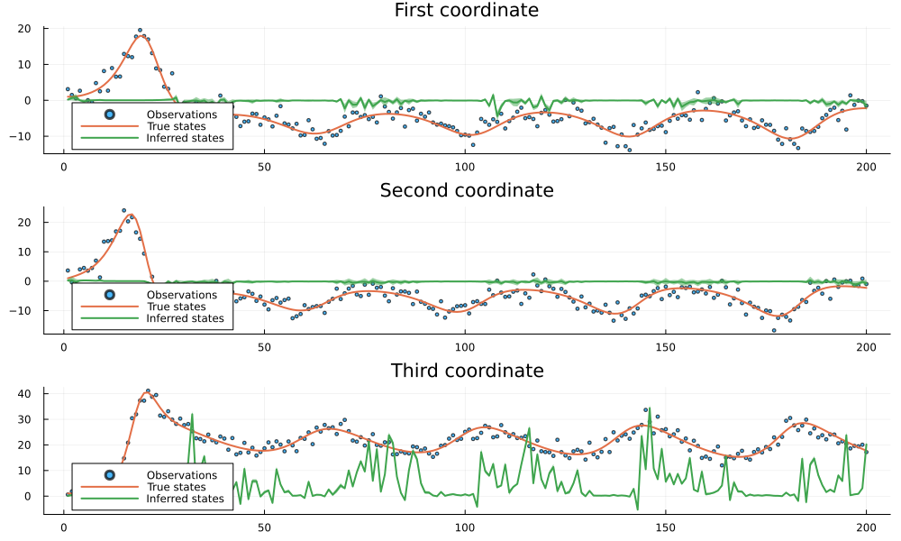
As we can see from the plots above, the inference results with an untrained neural network are essentially nonsense. The inferred states (green lines) fail to track the true states (orange lines) and instead produce arbitrary values with large uncertainty bands. This is expected since the untrained neural network generates random transition matrices that don't capture the actual dynamics of the system. The large discrepancy between the inferred and true states demonstrates why proper training of the neural network is necessary to achieve meaningful results.
Training the network
In this part, we use the Free Energy as the objective function to optimize the weights of our neural network. Free Energy is a variational inference objective that balances model fit with complexity. By minimizing Free Energy, we encourage the neural network to learn transition matrices that:
- Accurately predict the next state given the current state (reducing prediction error)
- Maintain appropriate uncertainty in the predictions
- Capture the underlying dynamics of the system without overfitting to noise
The optimization process iteratively updates the neural network weights using gradient descent. Because RxInfer.infer(...) is what computes the Free Energy — and Lux layers are pure functions — we can differentiate the whole pipeline with ForwardDiff, without touching any of RxInfer's internals.
# free energy objective to be optimized during training
function make_fe_tot_est(model, st, rebuild, data; Q = Q, B = B, R = R)
    function fe_tot_est(v)
        ps = rebuild(v)
        result = infer(
            model = ssm(As = get_matrices_from_neural_network(data, model, ps, st), Q = Q, B = B, R = R),
            data  = (y = data, ),
            returnvars = (x = KeepLast(), ),
            free_energy = true,
            session = nothing
        )
        return result.free_energy[end]
    end
end
make_fe_tot_est (generic function with 1 method)function train(model, ps, st, data; num_epochs = 500)
rule = Optimisers.Adam()
opt_state = Optimisers.setup(rule, ps)
_, rebuild = Optimisers.destructure(ps)
fe_tot_est_ = make_fe_tot_est(model, st, rebuild, data)
return run_epochs(rebuild, fe_tot_est_, opt_state, ps; num_epochs = num_epochs)
end
function run_epochs(rebuild::F, fe_tot_est::I, opt_state::S, ps::P; num_epochs::Int = 100) where {F, I, S, P}
print_each = num_epochs ÷ 10
start_time = time()
ps_current = ps
for epoch in 1:num_epochs
flat, _ = Optimisers.destructure(ps_current)
if epoch % print_each == 0
current_value = fe_tot_est(flat)
elapsed = time() - start_time
remaining = elapsed / epoch * (num_epochs - epoch)
println("Epoch $epoch/$num_epochs: Free Energy = $current_value, ETA: $(round(remaining; digits=1)) seconds")
end
grads = ForwardDiff.gradient(fe_tot_est, flat)
opt_state, ps_current = Optimisers.update(opt_state, ps_current, rebuild(grads))
end
total_time = time() - start_time
println("Finished in $(round(total_time; digits=1)) seconds")
return ps_current
endrun_epochs (generic function with 1 method)Now that we have defined our neural network architecture, dataset, and training functions, we can proceed with the training process. We'll train the neural network to learn the underlying dynamics of our state-space model from noisy observations. The training will optimize the free energy objective function using the Adam optimizer over multiple epochs. This process will allow the neural network to capture the non-linear relationships in the data, enabling more accurate state inference compared to traditional linear models. The following cell executes the training with 1000 epochs, which should provide sufficient iterations for convergence.
Note that unlike Flux, where Flux.update! mutates the layer in place, Lux parameters are stored in an immutable NamedTuple — so our train function returns the trained parameters rather than mutating them.
model, initial_ps, st = make_neural_network()

trained_ps = train(model, initial_ps, st, dataset.noisy_signal; num_epochs = 1000)
Epoch 100/1000: Free Energy = 24170.93445802461, ETA: 378.7 seconds
Epoch 200/1000: Free Energy = 22554.71504016765, ETA: 215.2 seconds
Epoch 300/1000: Free Energy = 20249.690550213167, ETA: 150.8 seconds
Epoch 400/1000: Free Energy = 15243.43215265174, ETA: 114.7 seconds
Epoch 500/1000: Free Energy = 5305.612489972754, ETA: 87.8 seconds
Epoch 600/1000: Free Energy = 1975.3465539892043, ETA: 66.4 seconds
Epoch 700/1000: Free Energy = 1565.5426626657077, ETA: 47.7 seconds
Epoch 800/1000: Free Energy = 1528.6284177456932, ETA: 30.8 seconds
Epoch 900/1000: Free Energy = 1515.1423138831697, ETA: 15.0 seconds
Epoch 1000/1000: Free Energy = 1510.1678087715945, ETA: 0.0 seconds
Finished in 146.7 seconds
(weight = Float32[-0.0013781071 0.0039143804 -0.005799058; -0.0037476972 0.
0001056586 -0.015720237; -0.00095079077 0.0046677166 -0.002318687], bias =
Float32[1.1312661, 1.2965654, 1.0732967])Now let's analyze the results of our neural network training. We'll visualize how well our trained model can infer the true states from noisy observations. The plots below will show the original noisy observations, the true underlying states, and our model's inferred states with confidence intervals. This comparison will help us evaluate the effectiveness of our neural network-based approach in capturing the non-linear dynamics of the system and filtering out noise.
trained_transition_matrices = get_matrices_from_neural_network(dataset.noisy_signal, model, trained_ps, st)

trained_result = infer(
    model = ssm(As = trained_transition_matrices, Q = Q, B = B, R = R),
    data  = (y = dataset.noisy_signal, ),
    returnvars = (x = KeepLast(), )
)

plot_coordinates(trained_result)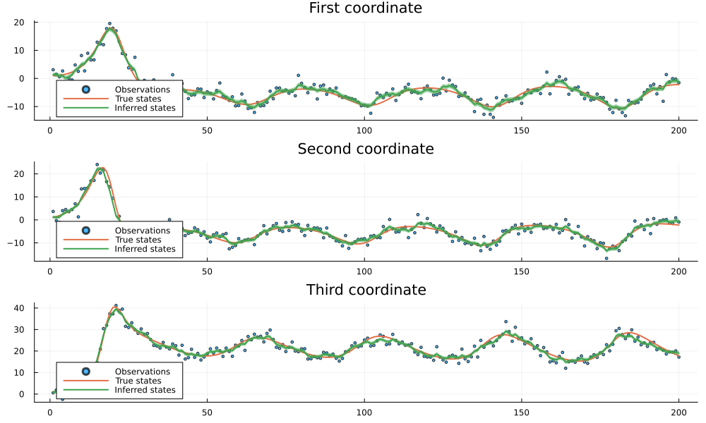
The results demonstrate the effectiveness of our neural network-based state-space model approach. Despite the significant noise present in the observations (shown as scattered points), our model successfully identifies the underlying hidden signal (shown by the inferred states line). The close alignment between the inferred states and the true states across all three coordinates indicates that the trained neural network has effectively learned the non-linear dynamics of the system. The narrow confidence bands (shown as ribbons) around the inferred states further suggest high confidence in the predictions. This example illustrates how combining neural networks with probabilistic state-space models can provide robust inference in scenarios with complex dynamics and noisy observations.
ix, iy, iz = zeros(n_points), zeros(n_points), zeros(n_points)

inferred_mean = mean.(trained_result.posteriors[:x])

# Extract coordinates
for i in 1:n_points
    # Inferred mean
    ix[i], iy[i], iz[i] = inferred_mean[i][1], inferred_mean[i][2], inferred_mean[i][3]
end

# Create three projection plots
p1 = scatter(rx, ry, label="Noisy observations", alpha=0.7, markersize=2, title = "X-Y Projection")
plot!(p1, gx, gy, label="True state", linewidth=2)
plot!(p1, ix, iy, label="Inferred Mean", linewidth=2)

p2 = scatter(rx, rz, label="Noisy observations", alpha=0.7, markersize=2, title = "X-Z Projection")
plot!(p2, gx, gz, label="True state", linewidth=2)
plot!(p2, ix, iz, label="Inferred Mean", linewidth=2)

p3 = scatter(ry, rz, label="Noisy observations", alpha=0.7, markersize=2, title = "Y-Z Projection")
plot!(p3, gy, gz, label="True state", linewidth=2)
plot!(p3, iy, iz, label="Inferred Mean", linewidth=2)

# Combine plots with improved layout
plot(p1, p2, p3, size=(900, 250), layout=(1,3), margin=5Plots.mm)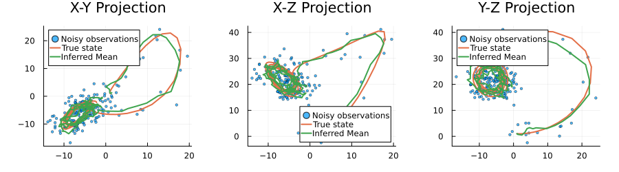
This example was automatically generated from a Jupyter notebook in the RxInferExamples.jl repository.
We welcome and encourage contributions! You can help by:
- Improving this example
- Creating new examples
- Reporting issues or bugs
- Suggesting enhancements
Visit our GitHub repository to get started. Together we can make RxInfer.jl even better! 💪
This example was executed in a clean, isolated environment. Below are the exact package versions used:
For reproducibility:
- Use the same package versions when running locally
- Report any issues with package compatibility
Status `/tmp/jl_9GI1bk/Project.toml`
⌅ [f6369f11] ForwardDiff v0.10.39
⌃ [b2108857] Lux v1.2.3
⌅ [3bd65402] Optimisers v0.3.4
  [91a5bcdd] Plots v1.41.6
  [86711068] RxInfer v5.1.0
  [860ef19b] StableRNGs v1.0.4
  [37e2e46d] LinearAlgebra v1.12.0
Info Packages marked with ⌃ and ⌅ have new versions available. Those with ⌃ may be upgradable, but those with ⌅ are restricted by compatibility constraints from upgrading. To see why use `status --outdated`