Conjugate-Computational Variational Message Passing (CVI)

using RxInfer, Random, LinearAlgebra, Plots, StableRNGs, ExponentialFamilyProjection
using Manopt: ConstantLength
include("call_closed_prod.jl")

In this notebook, the usage of Conjugate-Computational Variational Inference (CVI) will be described. The implementation of CVI follows the paper Probabilistic programming with stochastic variational message passing. RxInfer runs it with CVIProjection, an approximation method of the Delta node: it samples the inputs of a nonlinear function, pushes the samples through the function and projects the result onto an exponential family with ExponentialFamilyProjection.jl.

This notebook will first describe an example in which CVI is used, and then the requirements it places on a model.

An example: nonlinear dynamical system

A group of researchers is performing a tracking experiment on some moving object along a 1-dimensional trajectory. The object is moving at a constant velocity, meaning that its position increases constantly over time. However, the researchers do not have access to the absolute position $z_t$ at time $t$. Instead they have access to the observed squared distance $y_t$ between the object and some reference point $s$. Because of budget cuts, the servo moving the object and the measurement devices are quite outdated and therefore lead to noisy measurements:

# data generating process
nr_observations = 50
reference_point = 53
hidden_location = collect(1:nr_observations) + rand(StableRNG(124), NormalMeanVariance(0.0, sqrt(5)), nr_observations)
measurements = (hidden_location .- reference_point).^2 + rand(MersenneTwister(124), NormalMeanVariance(0.0, 5), nr_observations);

# plot hidden location and reference frame
p1 = plot(1:nr_observations, hidden_location, linewidth=3, legend=:topleft, label="hidden location")
hline!([reference_point], linewidth=3, label="reference point")
xlabel!("time [sec]"), ylabel!("location [cm]")

# plot measurements
p2 = scatter(1:nr_observations, measurements, linewidth=3, label="measurements")
xlabel!("time [sec]"), ylabel!("squared distance [cm2]")

plot(p1, p2, size=(1200, 500))

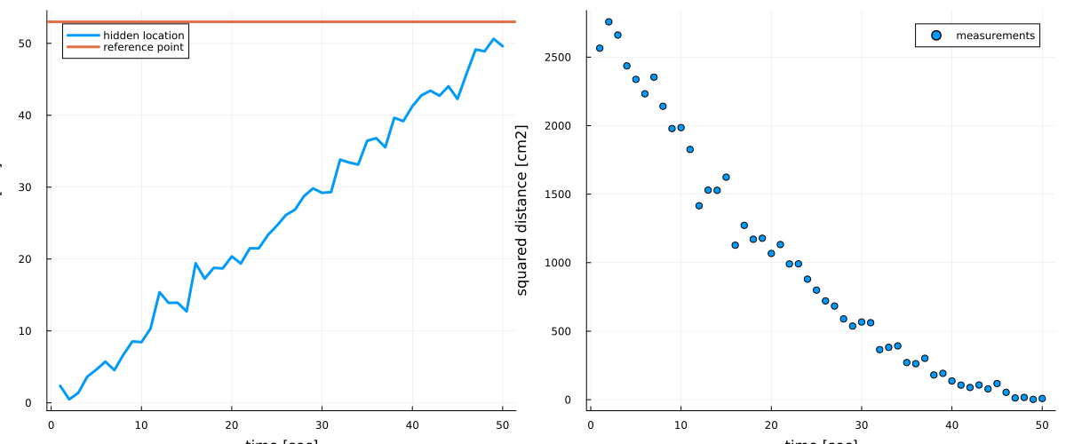
The researchers are interested in quantifying this noise and in tracking the unobserved location of the object. As a result of this uncertainty, the researchers employ a probabilistic modeling approach. They formulate the probabilistic model

\[\begin{aligned} p(\tau) & = \Gamma(\tau \mid \alpha_{\tau}, \beta_{\tau}),\\ p(\gamma) & = \Gamma(\gamma \mid \alpha_{\gamma}, \beta_{\gamma}),\\ p(z_t \mid z_{t - 1}, \tau) & = \mathcal{N}(z_t \mid z_{t - 1} + 1, \tau^{-1}),\\ p(y_t \mid z_t, \gamma) & = \mathcal{N}(y_t \mid (z_t - s)^2, \gamma^{-1}), \end{aligned}\]

where the researchers put priors on the process and measurement noise parameters, $\tau$ and $\gamma$, respectively. They do this, because they do not know the accuracy of their devices.

The researchers have recently heard of this cool probabilistic programming package RxInfer.jl. They decided to give it a try and create the above model as follows:

function compute_squared_distance(z)
    (z - reference_point)^2
end;

@model function measurement_model(y)

    # set priors on precision parameters
    τ ~ Gamma(shape = 0.01, rate = 0.01)
    γ ~ Gamma(shape = 0.01, rate = 0.01)
    
    # specify estimate of initial location
    z[1] ~ Normal(mean = 0, precision = τ)
    μ[1] := compute_squared_distance(z[1])
    y[1] ~ Normal(mean = μ[1], precision = γ)

    # loop over observations
    for t in 2:length(y)

        # specify state transition model
        z[t] ~ Normal(mean = z[t-1] + 1, precision = τ)

        # specify non-linear observation model
        μ[t] := compute_squared_distance(z[t])
        y[t] ~ Normal(mean = μ[t], precision = γ)
        
    end

end

But here is the problem, our compute_squared_distance function is already compelx enough such that the exact Bayesian inference is intractable in this model. But the researchers knew that the RxInfer.jl supports a various collection of approximation methods for exactly such cases. One of these approximations is called CVI. CVI allows us to perform probabilistic inference around the non-linear measurement function. In general, for any (non-)linear relationship y = f(x1, x2, ..., xN) CVI can be employed, by specifying the function f and by adding this relationship inside the @model macro as y ~ f(x1, x2, ...,xN). The @model macro will generate a factor node with node function p(y | x1, x2, ..., xN) = δ(y - f(x1, x2, ...,xN)).

The use of this non-linearity requires us to specify that we would like to use CVI. This can be done by specifying the node's algorithm with the @algorithm macro as:

projection_parameters = ProjectionParameters(stepsize = ConstantLength(1.0))

@algorithm function measurement_algorithm()
    compute_squared_distance() -> CVIProjection(in_prjparams = (in_1 = projection_parameters,), out_prjparams = projection_parameters)
end;

In general, for any (non-)linear function f(), CVI can be enabled with the @algorithm macro as:

@algorithm function model_algorithm(...)
    f() -> CVIProjection(args...)
end

See ?CVIProjection for more information about the args.... Each projection is a gradient descent over the parameters of the exponential family, and ProjectionParameters from ExponentialFamilyProjection.jl sets how it runs. With the default step length, ConstantLength(0.1), its 100 iterations do not travel far enough for this model, whose locations go up to 50, so here the steps have length 1. CVIProjection draws its samples from the random number generator of the inference, which is seeded below with the context option.

In our model, the z variables are connected to the non-linear node function. So in order to run probabilstic inference with CVI we need to enforce a constraint on the joint posterior distribution. Specifically, we need to create a factorization in which the variables that are directly connected to non-linearities are assumed to be independent from the rest of the variables.

In the above example, we will assume the following posterior factorization:

@constraints function measurement_constraints()
    q(z, μ, τ, γ) = q(z, μ)q(τ)q(γ)
    μ(z) :: CallClosedProd()
    q(z) :: CallClosedProd()
end;

The factorization can be explained by the set of two constraints, one for getting CVI to run, and one for assuming a mean-field factorization around the normal node as

@constraints function posterior_constraints()
    q(z, γ) = q(z)q(γ) # CVI
    q(z, τ) = q(z)q(τ) # the mean-field assumption around normal node
end

The two form constraints concern what CVIProjection sends back to z: its message is the projected marginal of z divided by the message that arrived from z, and it is left unevaluated. CallClosedProd, defined in call_closed_prod.jl next to this notebook, resolves the product of that division with the Gaussian messages on the other edges of z into one Gaussian, for the marginal q(z) and for the messages μ(z) that z sends on.

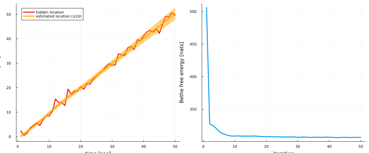
Because the engineers are using RxInfer.jl, they can automate the inference procedure. They track the inference performance using the Bethe free energy.

initialization = @initialization begin
    μ(z) = NormalMeanVariance(0, 5)
    μ(μ) = NormalMeanVariance(0, 5)
    q(z) = NormalMeanVariance(0, 5)
    q(μ) = NormalMeanVariance(0, 5)
    q(τ) = GammaShapeRate(1, 1)
    q(γ) = GammaShapeRate(1, 1)
end

results = infer(
    model = measurement_model(),
    data = (y = measurements,),
    iterations = 50,
    free_energy = true,
    returnvars = (z = KeepLast(),),
    constraints = measurement_constraints(),
    algorithm = measurement_algorithm(),
    initialization = initialization,
    options = (context = (rng = StableRNG(42),),),
)

Inference results:
  Posteriors       | available for (z)
  Free Energy:     | [557.811, 378.221, 370.387, 394.561, 395.947, 397.309,
 408.096, 398.641, 389.923, 403.484  …  403.175, 400.376, 405.155, 401.029,
 400.676, 390.583, 399.201, 406.749, 400.809, 399.676]

# plot estimates for location
p1 = plot(collect(1:nr_observations), hidden_location, label = "hidden location", legend=:topleft, linewidth=3, color = :red)
plot!(map(mean, results.posteriors[:z]), label = "estimated location (±2σ)", ribbon = map(x -> 2*std(x), results.posteriors[:z]), fillalpha=0.5, linewidth=3, color = :orange)
xlabel!("time [sec]"), ylabel!("location [cm]")

# plot Bethe free energy
p2 = plot(results.free_energy, linewidth=3, label = "")
xlabel!("iteration"), ylabel!("Bethe free energy [nats]")

plot(p1, p2, size = (1200, 500))

Requirements

There are several main requirements for the CVIProjection procedure to satisfy:

1. The out interface of the non-linearity must be independently factorized with respect to other variables in the model.
2. The messages on input interfaces (x1, x2, ..., xN) are required to be from the exponential family of distributions.
3. Where a variable on an input interface has more edges than the non-linearity and one other node, its marginal and its messages need a form constraint that resolves the unevaluated division, as CallClosedProd does above.

In RxInfer, you can satisfy the first requirement by using appropriate factor nodes (Normal, Gamma, Bernoulli, etc) and the second and third by specifying the @constraints macro. In general you can specify this procedure as

@model function model(...)
    ...
    y ~ f(x1, x2, ..., xN)
    ... ~ Node2(z1,..., y, zM) # some node that is using the out interface of the non-linearity
    ... 
end

@constraints function model_constraints()
    q(y, z1, ..., zM) = q(y)q(z1,...,zM)
    ...
end

@algorithm function model_algorithm(...)
    f() -> CVIProjection(args...)
end

Note that not all exponential family distributions are implemented.

Status `/tmp/jl_yh1YZg/Project.toml`
  [17f509fa] ExponentialFamilyProjection v3.4.0
  [0fc0a36d] Manopt v0.6.9
  [91a5bcdd] Plots v1.41.7
  [86711068] RxInfer v6.0.2
  [860ef19b] StableRNGs v1.1.0
  [37e2e46d] LinearAlgebra v1.13.0
  [9a3f8284] Random v1.11.0